Test Case: Binary Junction: Difference between revisions
(Added to the stress section and placed Figure 7) |
m (moved TOC) |
||
| (18 intermediate revisions by the same user not shown) | |||
| Line 1: | Line 1: | ||
=DDLab Binary Junction Tutorial= |
|||
'''Work in Progress''' |
|||
[[William Cash]]* and [[Seokwoo Lee]] |
|||
---- |
|||
| ⚫ | |||
__TOC__ |
|||
==Introduction== |
==Introduction== |
||
This tutorial will: |
This tutorial will: |
||
*Study the formation and dissociation of Lomer-Cottrell (binary) junctions in fcc crystals using |
*Study the formation and dissociation of Lomer-Cottrell (binary) junctions in fcc crystals using DDLab |
||
*Introduce running a batch of simulations, and calculating junction length and critical resolved shear stress to cause dissociation of the junction |
*Introduce running a batch of simulations, and calculating junction length and critical resolved shear stress to cause dissociation of the junction |
||
*Determine the dependence of junction length and critical stress on the initial orientation of the intersecting dislocations |
*Determine the dependence of junction length and critical stress at dissociation on the initial orientation of the intersecting dislocations |
||
*Determine the dependence of junction length and critical stress at dissociation on the initial length of the dislocations |
|||
*Illustrate the mobility of nodes at the intersection of glide planes in DDLab and ParaDiS |
|||
*Discuss any limitations. Physically the junction should be sessile. But in the simulation, the inner nodes of the junction segment are able to move. The end nodes of the junction are confined to the intersection line as they should. |
*Discuss any limitations. Physically the junction should be sessile. But in the simulation, the inner nodes of the junction segment are able to move. The end nodes of the junction are confined to the intersection line as they should. |
||
| Line 14: | Line 14: | ||
A copy of the input decks used in this tutorial can be downloaded from the link at the bottom of this page. |
A copy of the input decks used in this tutorial can be downloaded from the link at the bottom of this page. |
||
A tutorial for ParaDiS will be created in the future. |
|||
==Background== |
==Background== |
||
| Line 22: | Line 24: | ||
===Initial Orientation=== |
===Initial Orientation=== |
||
[[image:LC_formation.png|right|thumb|250px|Figure 1: Formation of a Lomer-Cottrell lock]] |
|||
These simulations are performed using the material constants for gold in order to conform with past computational and experimental results obtained by Madec et. al<ref name="Madec">''From Dislocation Junctions to Forest Hardening,'' Phys. Rev. Lett. 89 255508 (2002), R. Madec, B. Devincre, and L.P. Kubin</ref>, although any fcc metal could be used. In order to simplify the simulations, two dislocations with identical lengths, but on differing slip planes, are initially placed such that they intersect at their center. |
These simulations are performed using the material constants for gold in order to conform with past computational and experimental results obtained by Madec et. al<ref name="Madec">''From Dislocation Junctions to Forest Hardening,'' Phys. Rev. Lett. 89 255508 (2002), R. Madec, B. Devincre, and L.P. Kubin</ref>, although any fcc metal could be used. In order to simplify the simulations, two dislocations with identical lengths, but on differing slip planes, are initially placed such that they intersect at their center. The first dislocation glides on the <math>(\,1\,1\,1\,)</math> plane - henceforth referred to as dislocation 1. On the other hand, dislocation 2 glides on the <math>(\,1\,1\,\bar{1}\,)</math> plane. Both of these slip planes are part of the <math>\{\,1\,1\,1\,\}</math> slip system in fcc crystals. The dislocations have Burgers vectors of <math>\frac{1}{2}[\,1\,0\,\bar{1}\,]</math> and <math>\frac{1}{2}[\,0\,1\,1\,]</math>, respectively, regardless of their line direction <math>\mathbf{\xi}</math>. A Lomer-Cottrell junction could form at the intersection of these two planes, i.e. along the <math>[\,\bar{1}\,1\,0\,]</math> direction, if the conditions are correct, as shown in Figure 1. Thus, it is desired to determine the junction behavior at all combinations of line directions. |
||
If we consider all possible orientations |
If we consider all possible orientations of a straight dislocation of constant length and we take the origin to be the initial point of contact of the dislocations, we can define an end point (i.e. fixed node), <math>\mathbf{P}</math>, of the dislocation by a parametric equation of <math>\,\theta</math>: |
||
| ⚫ | |||
| Line 30: | Line 34: | ||
| ⚫ | where <math>\,R</math> is half the length of the dislocation; <math>\mathbf{u}</math> is a unit vector in the direction of the line of intersection, <math>[\,\bar{1}\,1\,0\,]</math> ; and <math>\mathbf{n}</math> is the unit normal of the glide plane. The vectors <math>\mathbf{P}</math> and <math>-\mathbf{P}</math> are then the end points of the dislocation. It is obvious from the equation that varying <math>\,\theta</math> from <math>[\,-\pi,\,\pi\,]</math> generates a circle on the glide plane. We have chosen to simulate 21 evenly distributed line orientations for both dislocations in this study. This results in a discretization for both dislocations shown in Figure 2, where the points represent one fixed node in each orientation and the initial line direction <math>\mathbf{\xi}</math> is taken as the vector from the origin to that point. <tt>LC_make_dis.m</tt> calculates the position of an end node of each dislocation in this manner using the following code: |
||
| ⚫ | |||
| ⚫ | where <math>R</math> is half the length of the dislocation; <math>\mathbf{u}</math> is a unit vector in the direction of the line of intersection, <math>[\,\bar{1}\,1\,0\,]</math> ; and <math>\mathbf{n}</math> is the unit glide plane |
||
<blockquote style="background: white; border: 0; padding: 1em; width: |
<blockquote style="background: white; border: 0; padding: 1em; width: 550px;"><pre> |
||
% Make dislocations |
% Make dislocations |
||
t |
t=[-1:0.1:1]*pi; |
||
%Creates dislocations on [1 1 1] |
%Creates end points of dislocations on [1 1 1] |
||
x1=dis_length/2*(-cos(t)/sqrt(2)-sin(t)/sqrt(6)); |
|||
y1=dis_length/2*(cos(t)/sqrt(2)-sin(t)/sqrt(6)); |
|||
z1=dis_length/2*(2*sin(t)/sqrt(6)); |
|||
%Creates dislocations on [1 1 -1] |
%Creates end points of dislocations on [1 1 -1] |
||
x2=dis_length/2*(-cos(t)/sqrt(2)+sin(t)/sqrt(6)); |
|||
y2=dis_length/2*(cos(t)/sqrt(2)+sin(t)/sqrt(6)); |
|||
z2=dis_length/2*(2*sin(t)/sqrt(6)); |
|||
%%Plots orientation circle plot seen in the Wiki |
|||
%figure(2) |
|||
%plot3(x,y,z,'-o', x1,y1,z1,'-o'); |
|||
%xlim([-2500 2500]);ylim([-2500 2500]);zlim([-2500 2500]); |
|||
%grid on |
|||
%view([30 -30 40]); |
|||
</pre></blockquote> |
</pre></blockquote> |
||
===Junction Length Calculation=== |
===Junction Length Calculation=== |
||
[[image:LC_zipped.jpg|right|thumb| |
[[image:LC_zipped.jpg|right|thumb|225px|Figure 3: Typical zipped binary junction]] |
||
| ⚫ | The length of the dislocation junction along the line of intersection is thought to be related to the strength of the Lomer-Cottrell lock. Therefore, we desire to calculate the junction length after the dislocations have been allowed to relax. We also want this calculation to be automated, because we hope to simulate 441 configurations. It is obvious from Figure 3 that the nodes at the ends of this "zipped" binary junction are unique in that they possess more than two arms. Calculating the length of the junction is as simple as finding the magnitude of the vector between the two free nodes possessing three or more arms from the first column of the <tt>linksconnect</tt> matrix. However, if the dislocations are oriented in such a way that junction formation is unfavorable, they could remain crossed at a single point, as illustrated in Figure 4. If there are less than two free nodes with three or more arms, then the junction length is zero. A simple algorithm in MATLAB is: |
||
| ⚫ | |||
| ⚫ | The length of the dislocation junction along the line of intersection is thought to be related to the strength of the Lomer-Cottrell lock. Therefore, we desire to calculate the junction length after the dislocations have been allowed to relax. We also want this calculation to be automated, because we hope to simulate 441 configurations. It is obvious from Figure |
||
<blockquote style="background: white; border: 0; padding: rem; width: |
<blockquote style="background: white; border: 0; padding: rem; width: 625px;"><pre> |
||
inter_nodes = find(-10^-2<rn(:,3) & rn(:,3)<10^-2 ); |
inter_nodes = find(-10^-2<rn(:,3) & rn(:,3)<10^-2 ); |
||
inter_nodes_seg = connectivity(inter_nodes,1); |
inter_nodes_seg = connectivity(inter_nodes,1); |
||
| Line 70: | Line 65: | ||
</pre></blockquote> |
</pre></blockquote> |
||
[[image: |
[[image:LC_cross.jpg|right|thumb|225px|Figure 4: Unfavorable junction orientation ]] |
||
| ⚫ | This algorithm works when the dislocations have only partially zipped a junction, which encompasses the majority of situations. However, if one of the dislocations is in the <math>[\,1\,\bar{1}\,0\,]</math> or <math>[\,\bar{1}\,1\,0\,]</math> direction, it is coincident with the intersection line and, thus, the dislocations have the possibility to fully zip the junction, as shown in Figure 5. In these situations a fixed end node is also the end node of the zipped junction. The end nodes of the junction now only possess two arms, because the fixed nodes were placed at the end of the dislocation. Therefore, the aforementioned algorithm would find the junction length to be zero, rather than the entire length of the original dislocation (4000). Since the fixed nodes possess a flag in <tt>rn</tt>, a simple improvement to the previous algorithm is: |
||
| ⚫ | |||
| ⚫ | This algorithm works when the dislocations have only partially zipped a junction, which encompasses the majority of situations. However, if one of the dislocations is in the <math>[\,1\,\bar{1}\,0\,]</math> or <math>[\,\bar{1}\,1\,0\,]</math> direction, it is coincident with the intersection line and, thus, the dislocations have the possibility to fully zip the junction, as shown in Figure |
||
| ⚫ | |||
fixed_nodes = find(rn(:,4)~=0); |
fixed_nodes = find(rn(:,4)~=0); |
||
inter_fixed_nodes = find(inter_coord(:,4)~=0); |
inter_fixed_nodes = find(inter_coord(:,4)~=0); |
||
| Line 81: | Line 75: | ||
</pre></blockquote> |
</pre></blockquote> |
||
[[image:LC_zipped_fully.jpg|right|thumb|225px|Figure 5: Fully zipped junction]] |
|||
This would add one to the connectivity of the end nodes such that the value of a zipped end node is three, which is detected as a junction end node. |
This would add one to the connectivity of the end nodes such that the value of a zipped end node is three, which is detected as a junction end node. |
||
[[image:LC_weird.jpg|right|thumb| |
[[image:LC_weird.jpg|right|thumb|225px|Figure 6: Repulsive coincident dislocations]] |
||
Unfortunately, this algorithm still fails to address when both dislocations overlap, i.e. they both lie along the intersection line. We know physically that the dislocations would combine to form a single dislocation if they are attractive. This is exactly what will happen in the simulations, because DDLab and ParaDiS both handle topological changes. Therefore, this junction length should be considered the entire length of the dislocation, but the previous algorithm would find it to be zero, because there are no nodes with more arms than they originally possessed. However, when the dislocations are repulsive the results in DDLab do not correspond to reality. The dislocations are not able to simply move apart, because their end nodes are pinned. The DDLab results for this situation can be seen in Figure |
Unfortunately, this algorithm still fails to address when both dislocations overlap, i.e. they both lie along the intersection line. We know physically that the dislocations would combine to form a single dislocation if they are attractive. This is exactly what will happen in the simulations, because DDLab and ParaDiS both handle topological changes. Therefore, this junction length should be considered the entire length of the dislocation, but the previous algorithm would find it to be zero, because there are no nodes with more arms than they originally possessed. However, when the dislocations are repulsive the results in DDLab do not correspond to reality. The dislocations are not able to simply move apart, because their end nodes are pinned. The DDLab results for this situation can be seen in Figure 6. In this case, only the end nodes will merge. An entirely different approach must be used to calculate junction length for these special cases. Initially, <tt>rn</tt> had four fixed nodes with a flag of 7; after the topological changes, there are only two fixed nodes, which is unique to these scenarios. In the case of repulsion the fixed nodes have two arms, while they only have one in attraction. These additions can be seen in <tt>LC_junction.m</tt> |
||
===Batch Execution=== |
===Batch Execution=== |
||
Executing a batch of 441 jobs in DDLab is |
Executing a batch of 441 jobs in DDLab is very simple due to the versatility of MATLAB. A separate script named <tt>LC_junction.m</tt> was created to call the DDLab input deck <tt>LC_relax.m</tt> for all iterations of the dislocations. Although it is possible to place the loops inside a DDLab input deck, it is best to keep the DDLab portions of the code separate from the other MATLAB scripts and retain the standard DDLab file layout.* <tt>LC_junction.m</tt> then stores the resulting nodal positions, <tt>rn</tt>; segment data, <tt>links</tt>; and junction length, <tt>junc_length</tt>, for all iterations in the MATLAB binary file <tt>LC_juction_data.mat</tt> for later analysis, and also as a restart point for the dissociation simulations explained in the next section. |
||
<nowiki>*</nowiki>It should also be noted that the input decks for ParaDiS cannot be modified from their usual format. |
|||
===Resolved Shear Stress Calculation=== |
===Resolved Shear Stress Calculation=== |
||
[[image:LC_shear_plane.png|right|thumb| |
[[image:LC_shear_plane.png|right|thumb|185px|Figure 7: Coordinate system for resolved shear stress]] |
||
After the dislocations are allowed to relax and form junctions. A shear stress is applied on the <math>(\,1\,1\,1\,)</math> plane in order to determine the resolved shear stress necessary to break the junction. Thus far, we have been using the Cartesian coordinate system with basis <math>\mathbf{e_1}=[\,1\,0\,0\,]</math>, <math>\mathbf{e_2}=[\,0\,1\,0\,]</math>, and <math>\mathbf{e_3}=[\,0\,0\,1\,]</math>. A stress transformation is needed in order to apply the shear directly on the <math>(\,1\,1\,1\,)</math> plane. The new orthogonal coordinate system was chosen as <math>\mathbf{e_1'}=[\,\bar{1}\,\bar{1}\,2\,]</math>, <math>\mathbf{e_2'}=[\,\bar{1}\,1\,0\,]</math>, and <math>\mathbf{e_3'}=[\,\bar{2}\,\bar{2}\,\bar{2}\,]</math>, as illustrated in Figure |
After the dislocations are allowed to relax and form junctions. A shear stress is applied on the <math>(\,1\,1\,1\,)</math> plane in order to determine the resolved shear stress necessary to break the junction. Thus far, we have been using the Cartesian coordinate system with basis <math>\mathbf{e_1}=[\,1\,0\,0\,]</math>, <math>\mathbf{e_2}=[\,0\,1\,0\,]</math>, and <math>\mathbf{e_3}=[\,0\,0\,1\,]</math>. A stress transformation is needed in order to apply the shear directly on the <math>(\,1\,1\,1\,)</math> plane. The new orthogonal coordinate system was chosen as <math>\mathbf{e_1'}=[\,\bar{1}\,\bar{1}\,2\,]</math>, <math>\mathbf{e_2'}=[\,\bar{1}\,1\,0\,]</math>, and <math>\mathbf{e_3'}=[\,\bar{2}\,\bar{2}\,\bar{2}\,]</math>, as illustrated in Figure 7. |
||
The stress transformation can be performed by the relation: |
The stress transformation can be performed by the relation: |
||
| Line 101: | Line 99: | ||
where <math>\mathbf{\sigma}</math> and <math>\mathbf{\sigma'}</math> are the stress tensor defined in the original and new coordinate systems, respectively. <math>\mathbf{Q}</math> is the transformation matrix, where its columns are the components of the basis <math>\mathbf{e'}</math> written in terms of the basis <math>\mathbf{e}</math>. If <math>\mathbf{e'}</math> and <math>\mathbf{e}</math> are chosen as orthonormal bases, then <math>\mathbf{Q}</math> is an orthogonal matrix consisting of directional cosines, and <math>\mathbf{Q^{-1}}</math> equals <math>\mathbf{Q^T}</math>. |
where <math>\mathbf{\sigma}</math> and <math>\mathbf{\sigma'}</math> are the stress tensor defined in the original and new coordinate systems, respectively. <math>\mathbf{Q}</math> is the transformation matrix, where its columns are the components of the basis <math>\mathbf{e'}</math> written in terms of the basis <math>\mathbf{e}</math>. If <math>\mathbf{e'}</math> and <math>\mathbf{e}</math> are chosen as orthonormal bases, then <math>\mathbf{Q}</math> is an orthogonal matrix consisting of directional cosines, and <math>\mathbf{Q^{-1}}</math> equals <math>\mathbf{Q^T}</math>. |
||
The resolved shear stress, <math>\,\tau_{13}</math> in basis <math>\mathbf{e'}</math> (Figure |
The resolved shear stress, <math>\,\tau_{13}</math> in basis <math>\mathbf{e'}</math> (Figure 7) is applied to the formed binary junction. This stress is transformed using the following algorithm in <tt>LC_stress.m</tt>: |
||
<blockquote style="background: white; border: 0; padding: rem; width: |
<blockquote style="background: white; border: 0; padding: rem; width: 525px;"><pre> |
||
%stress in coordinate system 2 |
%stress in coordinate system 2 |
||
sigma = [ 0 0 tau_13 |
sigma = [ 0 0 tau_13 |
||
| Line 125: | Line 123: | ||
</pre></blockquote> |
</pre></blockquote> |
||
[[image:LC_dissociation.png|right|thumb| |
[[image:LC_dissociation.png|right|thumb|250px|Figure 8: Dissociation of a Lomer-Cottrell lock]] |
||
This stress causes the junction to unzip by the bowing out of the dislocation arms, until a force equilibrium is reached. If the stress happens to be greater than the critical stress, then the binary junction will dissociate by fully unzipping the dislocation junction, as illustrated in Figure |
This stress causes the junction to unzip by the bowing out of the dislocation arms, until a force equilibrium is reached. If the stress happens to be greater than the critical stress, then the binary junction will dissociate by fully unzipping the dislocation junction, as illustrated in Figure 8. To avoid developing a complex iterative scheme to find the critical stress, this tutorial asks the user to input the magnitude of the applied stress until a satisfactory stress near the critical resolved shear stress is found. |
||
The strength of the junction has been shown to depend on the length of the dislocation arm, <math>\,l</math>, because the arms bow out like a Frank-Read Source, as shown in the sequence of Figure 8. The critical resolved shear stress to break the junction can be roughly obtained by the relationship: |
|||
<math>\tau_c\,\approx\,\frac{\mu b}{l}</math> |
|||
where <math>\,\mu</math> is the shear modulus and <math>\,b</math> is the magnitude of the Burgers vector. From the relation, it is obvious that dissociation can occur more easily with longer dislocation arms. If the initial length of the two dislocations increases, the resulting junction length increases. Also, the length of dislocation arms become longer (not shown), resulting in lower critical resolved shear stresses. |
|||
===Description of Files=== |
===Description of Files=== |
||
This section provides a brief description of all the files used in this tutorial and their hierarchy. The main bullets are the primary scripts, and the sub-bullets are the functions or scripts they call. |
This section provides a brief description of all the files used in this tutorial and their hierarchy. The main bullets are the primary scripts, and the sub-bullets are the functions or scripts they call. |
||
*'''<tt>LC_Junction.m</tt>'''- This script calculates the length of the junction formed between the two dislocations in the absence of stress, as described in the Junction Length Calculation section. It generates the surface plot of normalized junction length as a function of orientation shown in Figure |
*'''<tt>LC_Junction.m</tt>'''- This script calculates the length of the junction formed between the two dislocations in the absence of stress, as described in the Junction Length Calculation section. It generates the surface plot of normalized junction length as a function of orientation shown in Figure 9. It stores the final dislocation data and junction length (<tt>rn</tt>, <tt>links</tt>, and <tt>junc_length</tt>) in <tt>LC_junction_data.mat</tt>. |
||
**'''<tt>LC_make_dis.m</tt>'''- The script that generates the |
**'''<tt>LC_make_dis.m</tt>'''- The script that generates the coordinates of one fixed node for all 21 initial orientations of both dislocations from <math>\,-\pi</math> to <math>\,\pi</math>. The midpoint of all the dislocations is the origin |
||
**'''<tt>LC_relax.m</tt>'''- Script with the input deck for DDLab with zero applied stress. It requires <tt>D1</tt> and <tt>D2</tt>, one fixed node position for dislocations 1 and 2 respectively; and <tt>dis_length</tt>, the initial length of the dislocations, as inputs. |
**'''<tt>LC_relax.m</tt>'''- Script with the input deck for DDLab with zero applied stress. It requires <tt>D1</tt> and <tt>D2</tt>, one fixed node position for dislocations 1 and 2 respectively; and <tt>dis_length</tt>, the initial length of the dislocations, as inputs. |
||
**'''<tt>LC_junc_length.m</tt>'''- Function that calculates the length of the resulting binary junction. It takes the resulting <tt>rn</tt> and <tt>connectivity</tt> matrices from <tt>LC_relax.m</tt> as inputs and returns only junction length. |
**'''<tt>LC_junc_length.m</tt>'''- Function that calculates the length of the resulting binary junction. It takes the resulting <tt>rn</tt> and <tt>connectivity</tt> matrices from <tt>LC_relax.m</tt> as inputs and returns only junction length. |
||
*'''<tt> |
*'''<tt>LC_dissociate_orientation.m</tt>'''- This script determines the critical stress to dissociate a binary junction based on the orientation of the dislocations. The orientation angle of dislocation 1,<math>\,\phi_1</math> , equals <math>\frac{2\pi}{10}</math> and those of dislocation 2,<math>\,\phi_2</math> , are <math>\frac{\pi}{10}</math>, <math>\frac{2\pi}{10}</math>, and <math>\frac{3\pi}{10}</math>. The junction data is loaded from <tt>LC_junction_data.mat</tt>. The user inputs a guess at the critical shear stress in coordinate system 2 (see the Resolved Shear Stress Calculation section). The resulting critical shear stresses are plotted with <math>\,\phi_2</math> and junction length. It is best to start with a conservative guess to avoid having the dislocations dissociate and begin acting as Frank-Read sources, which is costly computationally. |
||
**'''<tt>LC_stress.m</tt>'''- Script with the DDLab input deck for the user specified <math>\,\tau_{13}</math> in coordinate system 2. It performs the stress transformation described in the Resolved Shear Stress Calculation section. It also requires that <tt>dis_length</tt>, the initial length of the dislocations prior to junction formation, is specified. |
**'''<tt>LC_stress.m</tt>'''- Script with the DDLab input deck for the user specified <math>\,\tau_{13}</math> in coordinate system 2. It performs the stress transformation described in the Resolved Shear Stress Calculation section. It also requires that <tt>dis_length</tt>, the initial length of the dislocations prior to junction formation, is specified. |
||
*'''<tt> |
*'''<tt>LC_dissociate_length.m</tt>'''- This script determines the critical stress to dissociate a binary junction based on the initial length of the dislocations. <math>\,\phi_1</math> and <math>\,\phi_2</math> are both chosen as <math>\frac{\pi}{10}</math>. The user inputs a guess at the critical shear stress in coordinate system 2 (see the Resolved Shear Stress Calculation section). The resulting critical shear stresses are plotted with junction length. |
||
**'''<tt>LC_relax.m</tt>'''- See above. |
**'''<tt>LC_relax.m</tt>'''- See above. |
||
**'''<tt>LC_junc_length.m</tt>'''- See above. |
**'''<tt>LC_junc_length.m</tt>'''- See above. |
||
| Line 148: | Line 154: | ||
==Results and Conclusions== |
==Results and Conclusions== |
||
===Junction Formation=== |
|||
| ⚫ | |||
Figure 9 shows the normalized resulting junction length between the dislocations under no external stresses. The junction length is highly dependent on both <math>\,\phi_1</math> and <math>\,\phi_2</math>. These results compare well with those published by Madec et. al.<ref name="Madec"/> Closer examination of the results reveals that reversing the line direction, <math>\mathbf{\xi}</math>, of both dislocations creates junctions with the same length. Although, the situations are not truly symmetric because the Burgers vectors do not flip, the lack of external stress means that the only forces are due to the interaction of the dislocations. Therefore in terms of junction formation, there is no difference between the junction of two dislocations and that of their opposites. For example, when <math>\phi_1=\frac{-9\pi}{10}</math> and <math>\phi_2=\frac{7\pi}{10}</math> their normalized junction length is 0.5862, which is the same as when <math>\phi_1=\frac{\pi}{10}</math> and <math>\phi_2=\frac{-3\pi}{10}</math>. This means the entire plot could have been generated by only varying <math>\,\phi_1</math> and <math>\,\phi_2</math> over the range <math>[\,0,\pi\,]</math>, thus cutting the number of trials in half. |
|||
===Junction Dissociation=== |
|||
Note: These are only preliminary results. Feel free to improve upon them. For the sake of time only a few junctions were manually dissociated. |
|||
The first comparisons in <tt>LC_dissociate_orientation.m</tt> are to see the effect of orientation on the junction strength. <math>\,\phi_1</math> is fixed at <math>\frac{\pi}{5}</math> and <math>\,\phi_2</math> is varied from <math>\frac{\pi}{10}</math> to <math>\frac{3\pi}{10}</math>. Figure 10 shows the critical resolved shear stress compared to <math>\,\phi_2</math>. The stress appears to decrease linearly with increasing angle, but the data are insufficient. The decrease in stress is expected, because the junction length decreases with increasing angle which means the that dislocation arms, <math>\,l</math>, are longer. Figure 11 compares the critical stress with the junction length. Again the relationship appears linear, but no conclusion can be made. |
|||
<gallery widths="225px" height="225px"> |
|||
image:LC_orientation_tc_vs_phi2.jpg|Figure 10: Critical stress compared with orientation angle |
|||
image:LC_orientation_tc_vs_length.jpg|Figure 11: Critical stress compared with junction length at different orientations |
|||
</gallery> |
|||
The effect of the initial dislocation length on the junction strength is studied in <tt>LC_dissociate_length.m</tt> The dislocation arm length, <math>\,l</math> should scale with junction length; thus, the longer dislocations should have lower critical resolved shear stresses. The junction length scales linearly with dislocation length, as illustrated in Figure 12. As expected, the junction strength decreases with increased increased junction length. Figure 13 shows the critical resolved shear stress appears to scale with <math>\frac{1}{l}</math>, which is predicted by the relationship in the Resolved Shear Stress Calculation section. |
|||
<gallery widths="225px" height="225px"> |
|||
image:LC_length_length_vs_length.jpg|Figure 12: Comparison of junction length with initial dislocation length |
|||
image:LC_length_tc_vs_length.jpg|Figure 13: Critical stress at various dislocation lengths |
|||
</gallery> |
|||
<font color="red">We can discuss in more detail which dislocation length is the controlling parameter for critical stress. Right now, the relaxed dislocation structure has five segments and their lengths are all related in this particular series of simulations. More simulations with different geometries are needed to determine which length is the controlling parameter.</font> |
|||
===Junction Dislocations in DDLab=== |
|||
[[image:LC_bowed.jpg|right|thumb|225px|Figure 14: Bowing of the binary junction should be avoided]] |
|||
Physically, the dislocation formed by the junction between two intersecting dislocations on differing slip planes is sessile, because it is composed of a partial dislocation in both slip planes. If one of the partials were to glide in its respective slip plane, it would force the other to climb. However in DDLab, the junction is formed using its normal split and merge topological changes, which means the nodes of the junction are not sessile. These operations enforce Burgers vector conservation, but calculate the slip plane by taking the cross product of the resulting Burgers vector and line direction. In the case of this tutorial, <math>\mathbf{b}=\frac{1}{2}[\,1\,1\,0\,]</math> and <math>\mathbf{n}=[\,0\,0\,1]</math> for the junction dislocation. The nodes at the end of the junction are constrained to only move along the line of intersection, because they are connected to segments in both slip planes. On the other hand, the nodes on the interior of the junction do not have such a restraint and are free to move in the <math>(\,0\,0\,1)</math> plane. If an external shear stress is applied to the junction, a situation such as that in Figure 14 can result. This bowing of the junction is clearly not physical and should be avoided. |
|||
==References== |
==References== |
||
<references/> |
<references/> |
||
[1] From Dislocation Junctions to Forest Hardening, Phys. Rev. Lett. 89 255508 (2002), R. Madec, B. Devincre, and L.P. Kubin |
|||
<font color="red">Currently, the references only show up automatically to logged in users. We are looking for a solution to this problem. For now we are just writing the references by hand.</font> |
|||
==Downloads== |
==Downloads== |
||
[[Media:LC_Junction_DDLab.tar.gz|LC_Junction_DDLab.tar.gz]] - DDLab tutorial files |
[[Media:LC_Junction_DDLab.tar.gz|LC_Junction_DDLab.tar.gz]] - DDLab tutorial files. (Note: best if extracted as a subdirectory of the DDLab Inputs folder) |
||
<font color="red">Note: there are currently some issues with the fcc mobility law in the latest release of DDLab (12/18/2007) that we hope to work out in the future. There is also a typo in <tt>mobfcc0.m</tt> involving <tt>BScrew</tt>, <tt>Bedge</tt>, etc. If you have any trouble resolving this issue please contact the author for a corrected version of the code.</font> |
|||
| ⚫ | |||
---- |
|||
[[image:LC_Junctions_DDLab.jpg|right|thumb|175px|[[help:contents|Figure X]]]] |
|||
<nowiki>*</nowiki> Please contact [[William Cash]] with any questions or concerns |
|||
[[image:LC_bowed.jpg|right|thumb|200px|[[help:contents|Figure X]]]] |
|||
Latest revision as of 00:34, 26 July 2008
DDLab Binary Junction Tutorial
William Cash* and Seokwoo Lee
Introduction
This tutorial will:
- Study the formation and dissociation of Lomer-Cottrell (binary) junctions in fcc crystals using DDLab
- Introduce running a batch of simulations, and calculating junction length and critical resolved shear stress to cause dissociation of the junction
- Determine the dependence of junction length and critical stress at dissociation on the initial orientation of the intersecting dislocations
- Determine the dependence of junction length and critical stress at dissociation on the initial length of the dislocations
- Discuss any limitations. Physically the junction should be sessile. But in the simulation, the inner nodes of the junction segment are able to move. The end nodes of the junction are confined to the intersection line as they should.
This tutorial assumes that the reader is familiar with the basics of DDLAB. New users should read DDLab_Manual_01 before proceeding.
A copy of the input decks used in this tutorial can be downloaded from the link at the bottom of this page.
A tutorial for ParaDiS will be created in the future.
Background
Plastic deformation of metals is usually governed by the motion of dislocations and their reactions, such as nucleation, pinning, and multiplication. One particularly important interaction occurs when two dislocations on different glide planes approach each other. These dislocations could either repel or attract each other depending on their Burgers vectors and orientations. If they are pulled together, the dislocations will combine in a way that minimizes their energy. This often results in the "zipping" of the dislocations along the line of intersection of the glide planes to form a junction known as a Lomer-Cottrell lock. These junctions have been shown to be a governing cause of strain hardening in fcc crystals.
Simulation Design
Initial Orientation

These simulations are performed using the material constants for gold in order to conform with past computational and experimental results obtained by Madec et. al[1], although any fcc metal could be used. In order to simplify the simulations, two dislocations with identical lengths, but on differing slip planes, are initially placed such that they intersect at their center. The first dislocation glides on the Failed to parse (SVG (MathML can be enabled via browser plugin): Invalid response ("Math extension cannot connect to Restbase.") from server "https://wikimedia.org/api/rest_v1/":): {\displaystyle (\,1\,1\,1\,)} plane - henceforth referred to as dislocation 1. On the other hand, dislocation 2 glides on the Failed to parse (SVG (MathML can be enabled via browser plugin): Invalid response ("Math extension cannot connect to Restbase.") from server "https://wikimedia.org/api/rest_v1/":): {\displaystyle (\,1\,1\,\bar{1}\,)} plane. Both of these slip planes are part of the Failed to parse (SVG (MathML can be enabled via browser plugin): Invalid response ("Math extension cannot connect to Restbase.") from server "https://wikimedia.org/api/rest_v1/":): {\displaystyle \{\,1\,1\,1\,\}} slip system in fcc crystals. The dislocations have Burgers vectors of Failed to parse (SVG (MathML can be enabled via browser plugin): Invalid response ("Math extension cannot connect to Restbase.") from server "https://wikimedia.org/api/rest_v1/":): {\displaystyle \frac{1}{2}[\,1\,0\,\bar{1}\,]} and Failed to parse (SVG (MathML can be enabled via browser plugin): Invalid response ("Math extension cannot connect to Restbase.") from server "https://wikimedia.org/api/rest_v1/":): {\displaystyle \frac{1}{2}[\,0\,1\,1\,]} , respectively, regardless of their line direction Failed to parse (SVG (MathML can be enabled via browser plugin): Invalid response ("Math extension cannot connect to Restbase.") from server "https://wikimedia.org/api/rest_v1/":): {\displaystyle \mathbf{\xi}} . A Lomer-Cottrell junction could form at the intersection of these two planes, i.e. along the Failed to parse (SVG (MathML can be enabled via browser plugin): Invalid response ("Math extension cannot connect to Restbase.") from server "https://wikimedia.org/api/rest_v1/":): {\displaystyle [\,\bar{1}\,1\,0\,]} direction, if the conditions are correct, as shown in Figure 1. Thus, it is desired to determine the junction behavior at all combinations of line directions.
If we consider all possible orientations of a straight dislocation of constant length and we take the origin to be the initial point of contact of the dislocations, we can define an end point (i.e. fixed node), Failed to parse (SVG (MathML can be enabled via browser plugin): Invalid response ("Math extension cannot connect to Restbase.") from server "https://wikimedia.org/api/rest_v1/":): {\displaystyle \mathbf{P}} , of the dislocation by a parametric equation of Failed to parse (SVG (MathML can be enabled via browser plugin): Invalid response ("Math extension cannot connect to Restbase.") from server "https://wikimedia.org/api/rest_v1/":): {\displaystyle \,\theta} :

Failed to parse (SVG (MathML can be enabled via browser plugin): Invalid response ("Math extension cannot connect to Restbase.") from server "https://wikimedia.org/api/rest_v1/":): {\displaystyle \mathbf{P} = R \cos(\theta)\mathbf{u} + R \sin(\theta)\mathbf{n} \times \mathbf{u}}
where Failed to parse (SVG (MathML can be enabled via browser plugin): Invalid response ("Math extension cannot connect to Restbase.") from server "https://wikimedia.org/api/rest_v1/":): {\displaystyle \,R}
is half the length of the dislocation; Failed to parse (SVG (MathML can be enabled via browser plugin): Invalid response ("Math extension cannot connect to Restbase.") from server "https://wikimedia.org/api/rest_v1/":): {\displaystyle \mathbf{u}}
is a unit vector in the direction of the line of intersection, Failed to parse (SVG (MathML can be enabled via browser plugin): Invalid response ("Math extension cannot connect to Restbase.") from server "https://wikimedia.org/api/rest_v1/":): {\displaystyle [\,\bar{1}\,1\,0\,]}
; and Failed to parse (SVG (MathML can be enabled via browser plugin): Invalid response ("Math extension cannot connect to Restbase.") from server "https://wikimedia.org/api/rest_v1/":): {\displaystyle \mathbf{n}}
is the unit normal of the glide plane. The vectors Failed to parse (SVG (MathML can be enabled via browser plugin): Invalid response ("Math extension cannot connect to Restbase.") from server "https://wikimedia.org/api/rest_v1/":): {\displaystyle \mathbf{P}}
and Failed to parse (SVG (MathML can be enabled via browser plugin): Invalid response ("Math extension cannot connect to Restbase.") from server "https://wikimedia.org/api/rest_v1/":): {\displaystyle -\mathbf{P}}
are then the end points of the dislocation. It is obvious from the equation that varying Failed to parse (SVG (MathML can be enabled via browser plugin): Invalid response ("Math extension cannot connect to Restbase.") from server "https://wikimedia.org/api/rest_v1/":): {\displaystyle \,\theta}
from Failed to parse (SVG (MathML can be enabled via browser plugin): Invalid response ("Math extension cannot connect to Restbase.") from server "https://wikimedia.org/api/rest_v1/":): {\displaystyle [\,-\pi,\,\pi\,]}
generates a circle on the glide plane. We have chosen to simulate 21 evenly distributed line orientations for both dislocations in this study. This results in a discretization for both dislocations shown in Figure 2, where the points represent one fixed node in each orientation and the initial line direction Failed to parse (SVG (MathML can be enabled via browser plugin): Invalid response ("Math extension cannot connect to Restbase.") from server "https://wikimedia.org/api/rest_v1/":): {\displaystyle \mathbf{\xi}}
is taken as the vector from the origin to that point. LC_make_dis.m calculates the position of an end node of each dislocation in this manner using the following code:
% Make dislocations
t=[-1:0.1:1]*pi;
%Creates end points of dislocations on [1 1 1]
x1=dis_length/2*(-cos(t)/sqrt(2)-sin(t)/sqrt(6));
y1=dis_length/2*(cos(t)/sqrt(2)-sin(t)/sqrt(6));
z1=dis_length/2*(2*sin(t)/sqrt(6));
%Creates end points of dislocations on [1 1 -1]
x2=dis_length/2*(-cos(t)/sqrt(2)+sin(t)/sqrt(6));
y2=dis_length/2*(cos(t)/sqrt(2)+sin(t)/sqrt(6));
z2=dis_length/2*(2*sin(t)/sqrt(6));
Junction Length Calculation

The length of the dislocation junction along the line of intersection is thought to be related to the strength of the Lomer-Cottrell lock. Therefore, we desire to calculate the junction length after the dislocations have been allowed to relax. We also want this calculation to be automated, because we hope to simulate 441 configurations. It is obvious from Figure 3 that the nodes at the ends of this "zipped" binary junction are unique in that they possess more than two arms. Calculating the length of the junction is as simple as finding the magnitude of the vector between the two free nodes possessing three or more arms from the first column of the linksconnect matrix. However, if the dislocations are oriented in such a way that junction formation is unfavorable, they could remain crossed at a single point, as illustrated in Figure 4. If there are less than two free nodes with three or more arms, then the junction length is zero. A simple algorithm in MATLAB is:
 inter_nodes = find(-10^-2<rn(:,3) & rn(:,3)<10^-2 );
 inter_nodes_seg = connectivity(inter_nodes,1);
 junc_end_nodes= find(inter_nodes_seg>2);
 if length(junc_end_nodes)<2
   junc_length(dis1_no,dis2_no)=0;
 else
   junc_length(dis1_no,dis2_no)=norm(inter_coord(junc_end_nodes(1),1:3)...
   -inter_coord(junc_end_nodes(2),1:3));
 end

This algorithm works when the dislocations have only partially zipped a junction, which encompasses the majority of situations. However, if one of the dislocations is in the or Failed to parse (SVG (MathML can be enabled via browser plugin): Invalid response ("Math extension cannot connect to Restbase.") from server "https://wikimedia.org/api/rest_v1/":): {\displaystyle [\,\bar{1}\,1\,0\,]} direction, it is coincident with the intersection line and, thus, the dislocations have the possibility to fully zip the junction, as shown in Figure 5. In these situations a fixed end node is also the end node of the zipped junction. The end nodes of the junction now only possess two arms, because the fixed nodes were placed at the end of the dislocation. Therefore, the aforementioned algorithm would find the junction length to be zero, rather than the entire length of the original dislocation (4000). Since the fixed nodes possess a flag in rn, a simple improvement to the previous algorithm is:
![{\displaystyle [\,1\,{\bar {1}}\,0\,]}](https://wikimedia.org/api/rest_v1/media/math/render/svg/0129bf5f18e40194a68f7cd1651c860e2b1226ba)
 fixed_nodes = find(rn(:,4)~=0);
 inter_fixed_nodes = find(inter_coord(:,4)~=0);
 ...
 inter_nodes_seg(inter_fixed_nodes)=inter_nodes_seg(inter_fixed_nodes)+1;

This would add one to the connectivity of the end nodes such that the value of a zipped end node is three, which is detected as a junction end node.

Unfortunately, this algorithm still fails to address when both dislocations overlap, i.e. they both lie along the intersection line. We know physically that the dislocations would combine to form a single dislocation if they are attractive. This is exactly what will happen in the simulations, because DDLab and ParaDiS both handle topological changes. Therefore, this junction length should be considered the entire length of the dislocation, but the previous algorithm would find it to be zero, because there are no nodes with more arms than they originally possessed. However, when the dislocations are repulsive the results in DDLab do not correspond to reality. The dislocations are not able to simply move apart, because their end nodes are pinned. The DDLab results for this situation can be seen in Figure 6. In this case, only the end nodes will merge. An entirely different approach must be used to calculate junction length for these special cases. Initially, rn had four fixed nodes with a flag of 7; after the topological changes, there are only two fixed nodes, which is unique to these scenarios. In the case of repulsion the fixed nodes have two arms, while they only have one in attraction. These additions can be seen in LC_junction.m
Batch Execution
Executing a batch of 441 jobs in DDLab is very simple due to the versatility of MATLAB. A separate script named LC_junction.m was created to call the DDLab input deck LC_relax.m for all iterations of the dislocations. Although it is possible to place the loops inside a DDLab input deck, it is best to keep the DDLab portions of the code separate from the other MATLAB scripts and retain the standard DDLab file layout.* LC_junction.m then stores the resulting nodal positions, rn; segment data, links; and junction length, junc_length, for all iterations in the MATLAB binary file LC_juction_data.mat for later analysis, and also as a restart point for the dissociation simulations explained in the next section.
*It should also be noted that the input decks for ParaDiS cannot be modified from their usual format.
Resolved Shear Stress Calculation

After the dislocations are allowed to relax and form junctions. A shear stress is applied on the Failed to parse (SVG (MathML can be enabled via browser plugin): Invalid response ("Math extension cannot connect to Restbase.") from server "https://wikimedia.org/api/rest_v1/":): {\displaystyle (\,1\,1\,1\,)} plane in order to determine the resolved shear stress necessary to break the junction. Thus far, we have been using the Cartesian coordinate system with basis Failed to parse (SVG (MathML can be enabled via browser plugin): Invalid response ("Math extension cannot connect to Restbase.") from server "https://wikimedia.org/api/rest_v1/":): {\displaystyle \mathbf{e_1}=[\,1\,0\,0\,]} , Failed to parse (SVG (MathML can be enabled via browser plugin): Invalid response ("Math extension cannot connect to Restbase.") from server "https://wikimedia.org/api/rest_v1/":): {\displaystyle \mathbf{e_2}=[\,0\,1\,0\,]} , and Failed to parse (SVG (MathML can be enabled via browser plugin): Invalid response ("Math extension cannot connect to Restbase.") from server "https://wikimedia.org/api/rest_v1/":): {\displaystyle \mathbf{e_3}=[\,0\,0\,1\,]} . A stress transformation is needed in order to apply the shear directly on the Failed to parse (SVG (MathML can be enabled via browser plugin): Invalid response ("Math extension cannot connect to Restbase.") from server "https://wikimedia.org/api/rest_v1/":): {\displaystyle (\,1\,1\,1\,)} plane. The new orthogonal coordinate system was chosen as Failed to parse (SVG (MathML can be enabled via browser plugin): Invalid response ("Math extension cannot connect to Restbase.") from server "https://wikimedia.org/api/rest_v1/":): {\displaystyle \mathbf{e_1'}=[\,\bar{1}\,\bar{1}\,2\,]} , Failed to parse (SVG (MathML can be enabled via browser plugin): Invalid response ("Math extension cannot connect to Restbase.") from server "https://wikimedia.org/api/rest_v1/":): {\displaystyle \mathbf{e_2'}=[\,\bar{1}\,1\,0\,]} , and Failed to parse (SVG (MathML can be enabled via browser plugin): Invalid response ("Math extension cannot connect to Restbase.") from server "https://wikimedia.org/api/rest_v1/":): {\displaystyle \mathbf{e_3'}=[\,\bar{2}\,\bar{2}\,\bar{2}\,]} , as illustrated in Figure 7.
The stress transformation can be performed by the relation:
Failed to parse (SVG (MathML can be enabled via browser plugin): Invalid response ("Math extension cannot connect to Restbase.") from server "https://wikimedia.org/api/rest_v1/":): {\displaystyle \mathbf{\sigma} = \mathbf{Q\,\sigma'\,Q^{-1}}}
where Failed to parse (SVG (MathML can be enabled via browser plugin): Invalid response ("Math extension cannot connect to Restbase.") from server "https://wikimedia.org/api/rest_v1/":): {\displaystyle \mathbf{\sigma}}
and Failed to parse (SVG (MathML can be enabled via browser plugin): Invalid response ("Math extension cannot connect to Restbase.") from server "https://wikimedia.org/api/rest_v1/":): {\displaystyle \mathbf{\sigma'}}
are the stress tensor defined in the original and new coordinate systems, respectively. Failed to parse (SVG (MathML can be enabled via browser plugin): Invalid response ("Math extension cannot connect to Restbase.") from server "https://wikimedia.org/api/rest_v1/":): {\displaystyle \mathbf{Q}}
is the transformation matrix, where its columns are the components of the basis Failed to parse (SVG (MathML can be enabled via browser plugin): Invalid response ("Math extension cannot connect to Restbase.") from server "https://wikimedia.org/api/rest_v1/":): {\displaystyle \mathbf{e'}}
written in terms of the basis Failed to parse (SVG (MathML can be enabled via browser plugin): Invalid response ("Math extension cannot connect to Restbase.") from server "https://wikimedia.org/api/rest_v1/":): {\displaystyle \mathbf{e}}
. If Failed to parse (SVG (MathML can be enabled via browser plugin): Invalid response ("Math extension cannot connect to Restbase.") from server "https://wikimedia.org/api/rest_v1/":): {\displaystyle \mathbf{e'}}
and Failed to parse (SVG (MathML can be enabled via browser plugin): Invalid response ("Math extension cannot connect to Restbase.") from server "https://wikimedia.org/api/rest_v1/":): {\displaystyle \mathbf{e}}
are chosen as orthonormal bases, then Failed to parse (SVG (MathML can be enabled via browser plugin): Invalid response ("Math extension cannot connect to Restbase.") from server "https://wikimedia.org/api/rest_v1/":): {\displaystyle \mathbf{Q}}
is an orthogonal matrix consisting of directional cosines, and Failed to parse (SVG (MathML can be enabled via browser plugin): Invalid response ("Math extension cannot connect to Restbase.") from server "https://wikimedia.org/api/rest_v1/":): {\displaystyle \mathbf{Q^{-1}}}
equals Failed to parse (SVG (MathML can be enabled via browser plugin): Invalid response ("Math extension cannot connect to Restbase.") from server "https://wikimedia.org/api/rest_v1/":): {\displaystyle \mathbf{Q^T}}
.
The resolved shear stress, Failed to parse (SVG (MathML can be enabled via browser plugin): Invalid response ("Math extension cannot connect to Restbase.") from server "https://wikimedia.org/api/rest_v1/":): {\displaystyle \,\tau_{13}} in basis Failed to parse (SVG (MathML can be enabled via browser plugin): Invalid response ("Math extension cannot connect to Restbase.") from server "https://wikimedia.org/api/rest_v1/":): {\displaystyle \mathbf{e'}} (Figure 7) is applied to the formed binary junction. This stress is transformed using the following algorithm in LC_stress.m:
%stress in coordinate system 2
sigma = [ 0    0  tau_13
          0    0  0
          tau_13  0  0 ] * 1e6;   %in Pa

%coordinate system 1 (cubic coordinate system)
e1p = [1 0 0]; e2p = [0 1 0]; e3p = [0 0 1];
e1p=e1p/norm(e1p); e2p=e2p/norm(e2p); e3p=e3p/norm(e3p);
%coordinate system 2
e1 =  [-1 -1 2]; e2  = [-1 1 0]; e3 = [-2 -2 -2];
e1=e1/norm(e1); e2=e2/norm(e2); e3=e3/norm(e3);

%rotation matrix
Q = [ dot(e1,e1p) dot(e2,e1p) dot(e3,e1p)
      dot(e1,e2p) dot(e2,e2p) dot(e3,e2p)
      dot(e1,e3p) dot(e2,e3p) dot(e3,e3p) ];

%Transform sigma into coordinate system 1
appliedstress = Q*sigma*Q';

This stress causes the junction to unzip by the bowing out of the dislocation arms, until a force equilibrium is reached. If the stress happens to be greater than the critical stress, then the binary junction will dissociate by fully unzipping the dislocation junction, as illustrated in Figure 8. To avoid developing a complex iterative scheme to find the critical stress, this tutorial asks the user to input the magnitude of the applied stress until a satisfactory stress near the critical resolved shear stress is found.
The strength of the junction has been shown to depend on the length of the dislocation arm, Failed to parse (SVG (MathML can be enabled via browser plugin): Invalid response ("Math extension cannot connect to Restbase.") from server "https://wikimedia.org/api/rest_v1/":): {\displaystyle \,l} , because the arms bow out like a Frank-Read Source, as shown in the sequence of Figure 8. The critical resolved shear stress to break the junction can be roughly obtained by the relationship:
Failed to parse (SVG (MathML can be enabled via browser plugin): Invalid response ("Math extension cannot connect to Restbase.") from server "https://wikimedia.org/api/rest_v1/":): {\displaystyle \tau_c\,\approx\,\frac{\mu b}{l}}
where Failed to parse (SVG (MathML can be enabled via browser plugin): Invalid response ("Math extension cannot connect to Restbase.") from server "https://wikimedia.org/api/rest_v1/":): {\displaystyle \,\mu}
is the shear modulus and Failed to parse (SVG (MathML can be enabled via browser plugin): Invalid response ("Math extension cannot connect to Restbase.") from server "https://wikimedia.org/api/rest_v1/":): {\displaystyle \,b}
is the magnitude of the Burgers vector. From the relation, it is obvious that dissociation can occur more easily with longer dislocation arms. If the initial length of the two dislocations increases, the resulting junction length increases. Also, the length of dislocation arms become longer (not shown), resulting in lower critical resolved shear stresses.
Description of Files
This section provides a brief description of all the files used in this tutorial and their hierarchy. The main bullets are the primary scripts, and the sub-bullets are the functions or scripts they call.
- LC_Junction.m- This script calculates the length of the junction formed between the two dislocations in the absence of stress, as described in the Junction Length Calculation section. It generates the surface plot of normalized junction length as a function of orientation shown in Figure 9. It stores the final dislocation data and junction length (rn, links, and junc_length) in LC_junction_data.mat.
- LC_make_dis.m- The script that generates the coordinates of one fixed node for all 21 initial orientations of both dislocations from Failed to parse (SVG (MathML can be enabled via browser plugin): Invalid response ("Math extension cannot connect to Restbase.") from server "https://wikimedia.org/api/rest_v1/":): {\displaystyle \,-\pi} to Failed to parse (SVG (MathML can be enabled via browser plugin): Invalid response ("Math extension cannot connect to Restbase.") from server "https://wikimedia.org/api/rest_v1/":): {\displaystyle \,\pi} . The midpoint of all the dislocations is the origin
- LC_relax.m- Script with the input deck for DDLab with zero applied stress. It requires D1 and D2, one fixed node position for dislocations 1 and 2 respectively; and dis_length, the initial length of the dislocations, as inputs.
- LC_junc_length.m- Function that calculates the length of the resulting binary junction. It takes the resulting rn and connectivity matrices from LC_relax.m as inputs and returns only junction length.
- LC_dissociate_orientation.m- This script determines the critical stress to dissociate a binary junction based on the orientation of the dislocations. The orientation angle of dislocation 1,Failed to parse (SVG (MathML can be enabled via browser plugin): Invalid response ("Math extension cannot connect to Restbase.") from server "https://wikimedia.org/api/rest_v1/":): {\displaystyle \,\phi_1}
, equals Failed to parse (SVG (MathML can be enabled via browser plugin): Invalid response ("Math extension cannot connect to Restbase.") from server "https://wikimedia.org/api/rest_v1/":): {\displaystyle \frac{2\pi}{10}}
and those of dislocation 2,Failed to parse (SVG (MathML can be enabled via browser plugin): Invalid response ("Math extension cannot connect to Restbase.") from server "https://wikimedia.org/api/rest_v1/":): {\displaystyle \,\phi_2}
, are Failed to parse (SVG (MathML can be enabled via browser plugin): Invalid response ("Math extension cannot connect to Restbase.") from server "https://wikimedia.org/api/rest_v1/":): {\displaystyle \frac{\pi}{10}}
, Failed to parse (SVG (MathML can be enabled via browser plugin): Invalid response ("Math extension cannot connect to Restbase.") from server "https://wikimedia.org/api/rest_v1/":): {\displaystyle \frac{2\pi}{10}}
, and Failed to parse (SVG (MathML can be enabled via browser plugin): Invalid response ("Math extension cannot connect to Restbase.") from server "https://wikimedia.org/api/rest_v1/":): {\displaystyle \frac{3\pi}{10}}
. The junction data is loaded from LC_junction_data.mat. The user inputs a guess at the critical shear stress in coordinate system 2 (see the Resolved Shear Stress Calculation section). The resulting critical shear stresses are plotted with Failed to parse (SVG (MathML can be enabled via browser plugin): Invalid response ("Math extension cannot connect to Restbase.") from server "https://wikimedia.org/api/rest_v1/":): {\displaystyle \,\phi_2}
and junction length. It is best to start with a conservative guess to avoid having the dislocations dissociate and begin acting as Frank-Read sources, which is costly computationally.
- LC_stress.m- Script with the DDLab input deck for the user specified Failed to parse (SVG (MathML can be enabled via browser plugin): Invalid response ("Math extension cannot connect to Restbase.") from server "https://wikimedia.org/api/rest_v1/":): {\displaystyle \,\tau_{13}} in coordinate system 2. It performs the stress transformation described in the Resolved Shear Stress Calculation section. It also requires that dis_length, the initial length of the dislocations prior to junction formation, is specified.
- LC_dissociate_length.m- This script determines the critical stress to dissociate a binary junction based on the initial length of the dislocations. Failed to parse (SVG (MathML can be enabled via browser plugin): Invalid response ("Math extension cannot connect to Restbase.") from server "https://wikimedia.org/api/rest_v1/":): {\displaystyle \,\phi_1}
and Failed to parse (SVG (MathML can be enabled via browser plugin): Invalid response ("Math extension cannot connect to Restbase.") from server "https://wikimedia.org/api/rest_v1/":): {\displaystyle \,\phi_2}
are both chosen as Failed to parse (SVG (MathML can be enabled via browser plugin): Invalid response ("Math extension cannot connect to Restbase.") from server "https://wikimedia.org/api/rest_v1/":): {\displaystyle \frac{\pi}{10}}
. The user inputs a guess at the critical shear stress in coordinate system 2 (see the Resolved Shear Stress Calculation section). The resulting critical shear stresses are plotted with junction length.
- LC_relax.m- See above.
- LC_junc_length.m- See above.
- LC_stress.m-See above.
Results and Conclusions
Junction Formation

Figure 9 shows the normalized resulting junction length between the dislocations under no external stresses. The junction length is highly dependent on both Failed to parse (SVG (MathML can be enabled via browser plugin): Invalid response ("Math extension cannot connect to Restbase.") from server "https://wikimedia.org/api/rest_v1/":): {\displaystyle \,\phi_1} and Failed to parse (SVG (MathML can be enabled via browser plugin): Invalid response ("Math extension cannot connect to Restbase.") from server "https://wikimedia.org/api/rest_v1/":): {\displaystyle \,\phi_2} . These results compare well with those published by Madec et. al.[1] Closer examination of the results reveals that reversing the line direction, Failed to parse (SVG (MathML can be enabled via browser plugin): Invalid response ("Math extension cannot connect to Restbase.") from server "https://wikimedia.org/api/rest_v1/":): {\displaystyle \mathbf{\xi}} , of both dislocations creates junctions with the same length. Although, the situations are not truly symmetric because the Burgers vectors do not flip, the lack of external stress means that the only forces are due to the interaction of the dislocations. Therefore in terms of junction formation, there is no difference between the junction of two dislocations and that of their opposites. For example, when Failed to parse (SVG (MathML can be enabled via browser plugin): Invalid response ("Math extension cannot connect to Restbase.") from server "https://wikimedia.org/api/rest_v1/":): {\displaystyle \phi_1=\frac{-9\pi}{10}} and Failed to parse (SVG (MathML can be enabled via browser plugin): Invalid response ("Math extension cannot connect to Restbase.") from server "https://wikimedia.org/api/rest_v1/":): {\displaystyle \phi_2=\frac{7\pi}{10}} their normalized junction length is 0.5862, which is the same as when Failed to parse (SVG (MathML can be enabled via browser plugin): Invalid response ("Math extension cannot connect to Restbase.") from server "https://wikimedia.org/api/rest_v1/":): {\displaystyle \phi_1=\frac{\pi}{10}} and Failed to parse (SVG (MathML can be enabled via browser plugin): Invalid response ("Math extension cannot connect to Restbase.") from server "https://wikimedia.org/api/rest_v1/":): {\displaystyle \phi_2=\frac{-3\pi}{10}} . This means the entire plot could have been generated by only varying Failed to parse (SVG (MathML can be enabled via browser plugin): Invalid response ("Math extension cannot connect to Restbase.") from server "https://wikimedia.org/api/rest_v1/":): {\displaystyle \,\phi_1} and Failed to parse (SVG (MathML can be enabled via browser plugin): Invalid response ("Math extension cannot connect to Restbase.") from server "https://wikimedia.org/api/rest_v1/":): {\displaystyle \,\phi_2} over the range Failed to parse (SVG (MathML can be enabled via browser plugin): Invalid response ("Math extension cannot connect to Restbase.") from server "https://wikimedia.org/api/rest_v1/":): {\displaystyle [\,0,\pi\,]} , thus cutting the number of trials in half.
Junction Dissociation
Note: These are only preliminary results. Feel free to improve upon them. For the sake of time only a few junctions were manually dissociated.
The first comparisons in LC_dissociate_orientation.m are to see the effect of orientation on the junction strength. Failed to parse (SVG (MathML can be enabled via browser plugin): Invalid response ("Math extension cannot connect to Restbase.") from server "https://wikimedia.org/api/rest_v1/":): {\displaystyle \,\phi_1} is fixed at Failed to parse (SVG (MathML can be enabled via browser plugin): Invalid response ("Math extension cannot connect to Restbase.") from server "https://wikimedia.org/api/rest_v1/":): {\displaystyle \frac{\pi}{5}} and Failed to parse (SVG (MathML can be enabled via browser plugin): Invalid response ("Math extension cannot connect to Restbase.") from server "https://wikimedia.org/api/rest_v1/":): {\displaystyle \,\phi_2} is varied from Failed to parse (SVG (MathML can be enabled via browser plugin): Invalid response ("Math extension cannot connect to Restbase.") from server "https://wikimedia.org/api/rest_v1/":): {\displaystyle \frac{\pi}{10}} to Failed to parse (SVG (MathML can be enabled via browser plugin): Invalid response ("Math extension cannot connect to Restbase.") from server "https://wikimedia.org/api/rest_v1/":): {\displaystyle \frac{3\pi}{10}} . Figure 10 shows the critical resolved shear stress compared to Failed to parse (SVG (MathML can be enabled via browser plugin): Invalid response ("Math extension cannot connect to Restbase.") from server "https://wikimedia.org/api/rest_v1/":): {\displaystyle \,\phi_2} . The stress appears to decrease linearly with increasing angle, but the data are insufficient. The decrease in stress is expected, because the junction length decreases with increasing angle which means the that dislocation arms, Failed to parse (SVG (MathML can be enabled via browser plugin): Invalid response ("Math extension cannot connect to Restbase.") from server "https://wikimedia.org/api/rest_v1/":): {\displaystyle \,l} , are longer. Figure 11 compares the critical stress with the junction length. Again the relationship appears linear, but no conclusion can be made.
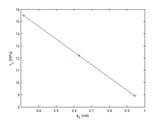
Figure 10: Critical stress compared with orientation angle
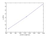
Figure 11: Critical stress compared with junction length at different orientations


The effect of the initial dislocation length on the junction strength is studied in LC_dissociate_length.m The dislocation arm length, Failed to parse (SVG (MathML can be enabled via browser plugin): Invalid response ("Math extension cannot connect to Restbase.") from server "https://wikimedia.org/api/rest_v1/":): {\displaystyle \,l} should scale with junction length; thus, the longer dislocations should have lower critical resolved shear stresses. The junction length scales linearly with dislocation length, as illustrated in Figure 12. As expected, the junction strength decreases with increased increased junction length. Figure 13 shows the critical resolved shear stress appears to scale with Failed to parse (SVG (MathML can be enabled via browser plugin): Invalid response ("Math extension cannot connect to Restbase.") from server "https://wikimedia.org/api/rest_v1/":): {\displaystyle \frac{1}{l}} , which is predicted by the relationship in the Resolved Shear Stress Calculation section.
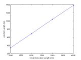
Figure 12: Comparison of junction length with initial dislocation length
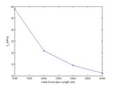
Figure 13: Critical stress at various dislocation lengths


We can discuss in more detail which dislocation length is the controlling parameter for critical stress. Right now, the relaxed dislocation structure has five segments and their lengths are all related in this particular series of simulations. More simulations with different geometries are needed to determine which length is the controlling parameter.
Junction Dislocations in DDLab

Physically, the dislocation formed by the junction between two intersecting dislocations on differing slip planes is sessile, because it is composed of a partial dislocation in both slip planes. If one of the partials were to glide in its respective slip plane, it would force the other to climb. However in DDLab, the junction is formed using its normal split and merge topological changes, which means the nodes of the junction are not sessile. These operations enforce Burgers vector conservation, but calculate the slip plane by taking the cross product of the resulting Burgers vector and line direction. In the case of this tutorial, Failed to parse (SVG (MathML can be enabled via browser plugin): Invalid response ("Math extension cannot connect to Restbase.") from server "https://wikimedia.org/api/rest_v1/":): {\displaystyle \mathbf{b}=\frac{1}{2}[\,1\,1\,0\,]} and Failed to parse (SVG (MathML can be enabled via browser plugin): Invalid response ("Math extension cannot connect to Restbase.") from server "https://wikimedia.org/api/rest_v1/":): {\displaystyle \mathbf{n}=[\,0\,0\,1]} for the junction dislocation. The nodes at the end of the junction are constrained to only move along the line of intersection, because they are connected to segments in both slip planes. On the other hand, the nodes on the interior of the junction do not have such a restraint and are free to move in the Failed to parse (SVG (MathML can be enabled via browser plugin): Invalid response ("Math extension cannot connect to Restbase.") from server "https://wikimedia.org/api/rest_v1/":): {\displaystyle (\,0\,0\,1)} plane. If an external shear stress is applied to the junction, a situation such as that in Figure 14 can result. This bowing of the junction is clearly not physical and should be avoided.
References
[1] From Dislocation Junctions to Forest Hardening, Phys. Rev. Lett. 89 255508 (2002), R. Madec, B. Devincre, and L.P. Kubin
Currently, the references only show up automatically to logged in users. We are looking for a solution to this problem. For now we are just writing the references by hand.
Downloads
LC_Junction_DDLab.tar.gz - DDLab tutorial files. (Note: best if extracted as a subdirectory of the DDLab Inputs folder)
Note: there are currently some issues with the fcc mobility law in the latest release of DDLab (12/18/2007) that we hope to work out in the future. There is also a typo in mobfcc0.m involving BScrew, Bedge, etc. If you have any trouble resolving this issue please contact the author for a corrected version of the code.
LC_lock.pdf. - Past version of this tutorial. (Note: There are some errors associated with the junction length calculation and the codes have been significantly modified)
* Please contact William Cash with any questions or concerns