Test Case: Frank-Read Source

Introduction

Frank-Read source is a type of dislocation multiplication mechanism. Consider a segment whose ends are pinned (corresponding to nodes in a network, precipitates, or sites where the dislocation leaves the glide plane). Under a certain applied stress the segment bows out by glide. As bow-out proceeds, the radius of curvature of the line decreases and the line-tension forces tending to restore the line to a straight configuration increase. For stress less than a critical value, a metastable equilibrium configuration is attained, in which the line-tension force balances that caused by the applied stress. For the large bow-out case, following equilibrium condition holds:

$b\mathbf{\sigma} = \frac{\mathbb{S}}{r}=\frac{\mu b^2}{4\pi r\left( 1-\nu\right)} \left \{ \left [ 1- \frac{\nu}{2} \left ( 3-4 \cos^2\beta \right ) \right ] \mathrm{ln} \frac{L}{\rho} -1 + \frac{\nu}{2} \right \}$

(Hirth-Lothe, p. 752)

where r is the radius of the loop. The radius of the curvature is a minimum when $r = L / 2$ . Hence the maximum stress for which local equilibrium is possible is given by the equation above with $r = L / 2$ . For the typical case that $L = 10 3 ρ$ and $μ = 0.33$ , the critical stress for a dislocation initially pure edge and pure screw, respectively, is $σ * = 0.5μ b / L$ and $σ * = 1.5μ b / L$ .

When the net local resolved shear stress( the applied stress plus the internal stresses) exceeds $σ *$ , the loop has no stable equilibrium configuration but passes through the successive positions. Provided that the expanding loop neither jogs out of the original glide plane because of intersections with other dislocations nor is obstructed from rotating about the pinning point, it will annihilate over a portion of its length, creating a complete closed loop and restoring the original configuration. A sequence of loops then continues to form from the source until sufficient internal stresses are generated for the net resolved shear stress at the source to drop below $σ *$ .

To compare the analytic result with DDLab simulation, we need to use the relation $ρ = r c / 2$ . According to the non-singular continuum theory of dislocation (JMPS 54, 561-587, 2006), the energy of a circular prismatic dislocation loop is

$E = 2 \pi R \frac{\mu b^2}{4 \pi (1-\nu)} \left( \ln \frac{8 R}{r_c} - 1 \right) + O\left(\frac{a^2}{R^2}\right)$

According to Hirth and Lothe, the energy of the same loop is,

$E = 2 \pi R \frac{\mu b^2}{4 \pi (1-\nu)} \left( \ln \frac{4 R}{\rho} - 1 \right)$

Therefore $\rho = \frac{r_c}{2}$

Reference: J. P. Hirth and J. Lothe, Theory of Dislocations", 2nd ed. (Wiley, New York, 1982)

DDLab Input Parameter

DDLab has included a sample Frank-Read Source input file in its latest version (2008 January) at ~/Inputs/input_frank_read.m. Following is a brief introduction to some parameters important to Frank-Read source test.

1. rn--it gives the initial coordinations of nodes. The default setting is a straight dislocation line pinned (tag=7) at (1200,1200,1200) and (-1200,-1200,-1200) with a mobile (tag=0) node in the middle, (0,0,0). Of course, 1200 can be substituted into arbitrary numbers when we investigate the influence of initial segmental length.

2. links--a data structure which gives the information of dislocation segment connectivity, burgers vectors( [0.5 0.5 0.5] default ) and glide planes (-1,1,0) default ).

3. totalsteps--number of cycles that are run for completion of dd3d command. It should be large enough to secure dislocation configuration has arrived at its equilibrium configuration, for example, 1000 or above.

4. appliedstress--external applied stress in the form of 3*3 symmetric tensor. Peach-Koehler formula will be needed to give the exact force on each segment, i.e.

$\mathit{\mathbf{f}} ^{PK} (x)=(\mathbf{\sigma} (x) \cdot \mathit{\mathbf{b}} ) \times \mathbf{\xi} (x)$

We need to use this formula to give F-R $σ *$ under certain appliedstress.

5. a--dislocation core radius used for non-singular force calculation, sometimes written as $r c$ .

6. plotfreq--number of cycles between monitered node write statements, higher number makes observation simpler. When the dislocation line goes beyond plotting limits, simply Increasing plim can provide a better view.

7. lmin and lmax -- minimum and maximum length of a dislocation segment for remeshing. The shorter segments are, the smoother dislocation line becomes.

8. mobility --mobility law based on which dislocation responds to forces (mobbcc0 for BCC, which is the default setting; mobfcc1 for FCC). For FCC crystals, glide plane is uniquely defined rather BCC, i.e. dislocation motion is confined to a preferred plane.

We can manipulate these parameters to investigate Frank-Read Sources via DDLab.

F-R Test

1. Criteria to define $σ *$

In the case of Frank-Read source, It is difficult to give a quantitative definition on critical applied stress. When totalsteps is large enough, the bowing process will eventually stop unless that critical stress has been reached. Let's define a certain geometric configuration beyond which the dislocation line becomes unstable and keeps growing, even forming loops. When such configuration is formed, we denote the current external applied stress as the critical one. It is convenient to use maximum distance criteria, that we can extract the coordinates of all nodes from rn and find out the maximum distance from the center of initial dislocation line. If the maximum distance exceeds an empirical value, let's say, L, which is the length of initial dislocation line, we can regard the configuration as "critical" and determine the critical stress, $σ *$ . Several trials have proven that L is a safe one. As long as totalsteps is large enough, 2L, 4L etc will also work well.

2. Basic settings

The initial dislocation line is pinned at (-l,-l,-l) ,(l, l, l). (0, 0, 0) is a mobile node at the center.

We can change any parameter before running dd3d.m. Simple test cases have shown that when l ranges from 1,000 to 10,000, the external applied stress is at the order of $10 - 4$ .


rn    = [ 1000    1000   1000     7;
	 -1000   -1000  -1000     7;     %pinned at two ends
	     0       0      0     0];    %mobile node in the middle
links = [1 3 0.5 0.5 0.5 -1 1 0;
	 3 2 0.5 0.5 0.5 -1 1 0];      %burgers vector [0.5 0.5 0.5], glide plane (-1 1 0)

MU = 1;
NU = 0.305;   %elasticity constants for isotropic media

maxconnections=8;
lmax = 1000;
lmin = 200;     % fixed lmax and lmin for all cases
areamin=lmin*lmin*sin(60/180*pi)*0.5; 
areamax=20*areamin;

a=lmin/sqrt(3)*0.5;     %defined in terms of lmin
Ec = MU/(4*pi)*log(a/0.1);   %Ec=0 when compared with analytical expression
totalsteps=200;   %enough for rough estimations
dt0=1e7;  
mobility='mobfcc1';   %FCC mobility law

%Drag (Mobility) parameters
Bscrew=1e0;
Bedge=1e0;
Beclimb=1e2;
Bline=1.0e-4*min(Bscrew,Bedge);

integrator='int_trapezoid';
rann = 0.5*a;       
rntol = 0.5*rann;    
doremesh=1;
docollision=1;
doseparation=1;
elasticinteraction=1;     %line tension model when this is zero
plotfreq=1;       
plim=10000;         
appliedstress =1e-3.*[2 0 1; 0 2 -1; 1 -1 0];   % a value times a stress tensor
viewangle=[45 -45];
printfreq=1;       %set as 10 for better view
printnode=3;
rmax=100;

3. Algorithm

The critical stress is determined digit by digit. Assuming the critical externally applied stress is 2.35e-4 times a matrix A, to determine the first digit, simulation is run for 400 steps when the applied stress is 1e-4*A. The stress will be increased by 1e-4*A unless the maximum criteria is not reached. We will see, the first digit is 3. As for the second digit, the initial applied stress starts from 2.1e-4*A and simulation is run for 1000 steps. In the similar manner, 2.2e-4*A will be applied if critical criteria is not met. Finally, the second digit is 4. To determine the third digit, simulation starts at 2.31e-4*A...Of course, the matrix A and totalsteps are subject to change. More simulation steps will be needed when the stress increase is smaller, i.e. better accuracy. For detailed coding, please refer to crstrfr.m.

4. Investigation

4.1. L dependence

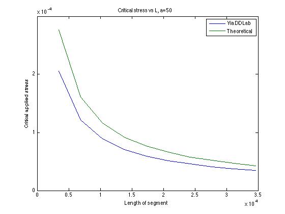
Based on the maximum distance criteria, we can easily determine the critical applied stress for different initial straight line lengths. Here is a graph showing the relationship between $σ c$ and L at a=50.

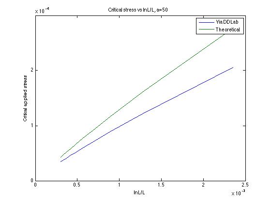
According to the formula, there is a linear relation between the critical stress and segment length L, which was also proven by numerical results.

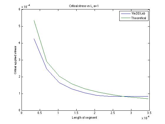
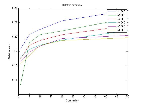
The relative error decreases from 0.26 to 0.20 when the initial segment coordinate parameter l goes from 1000 to 10,000; however, the error can't be negligible. Better convergence should occur at a smaller a value. Numerical tests shows that, when a=1, relative error decreases from 0.20 to 0.18 when l goes from 1000 to 6000. Lower error is expected for longer segments.

Longer simulation time can help eliminate the intersections at large l.

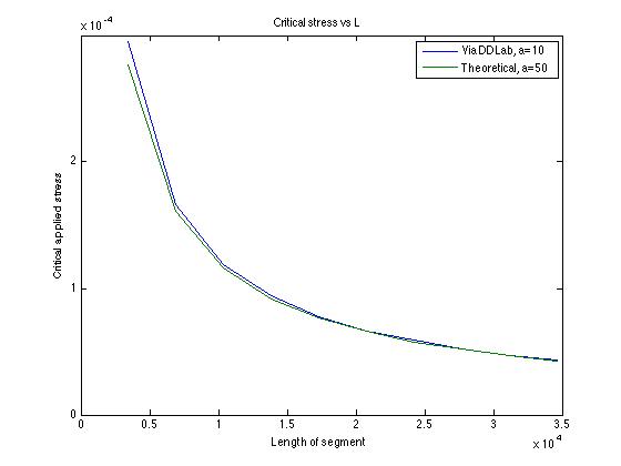
A interesting phenomenon is that numerical result for a/5 well fits analytical result for a. Relative error goes to 0.01 when l goes to 10,000.

It shows that analytical result will be more accurate at smaller a/L ratio.

4.2. a dependence

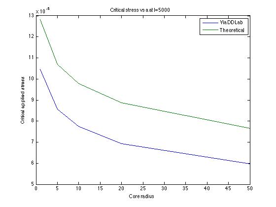
When a varies from 1 to 50 and l is fixed at 5000, numerical results are given, shown in following figures

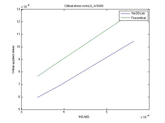
Same as the formula, the critical stress has a linear dependence on ln(L/a)/L

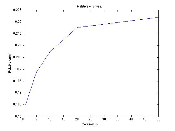
We can see the decrease in relative error.

When the length of initial segment increases, relative error seems to decrease when a approaches 0.

4.3. lmax influence

Above results are based on the setting that lmax=l, lmin=l/10 other than the default lmax=1000, limin=200. Though the dislocation line is less smoother, numerical results are the same for the case l=5000. For computation simplicity, we can set lmax and lmin proportional to l and get reasonable results.

Conclusion

After conducting several test cases of Frank-Read Source using DDLab, we have shown:

1, The critical stress is linearly dependent on ln(L/a)/L;

2. Numerical results are closer to theoretical ones at small a and large L.

3. Numerical critical stress for a/5 well fits theoretical results for a

Some of the plots above will be updated when more accurate data are available for a=1 (or less) and L>6000.

Contents

Introduction

DDLab Input Parameter

F-R Test

Conclusion