Manual 07 for MD++
Computing Elastic Constants

Keonwook Kang and Wei Cai

Nov 28 , 2007

Elastic constants are physical properties of crystals to relate the mechanical response to the material deformation (i.e. stress and strain) within elastic regime. To calculate the elastic constants is one simple way of validating a potential model. There are two methods to compute elastic constants: one is to monitor (Virial) stress and the other is to monitor strain energy as a function of the applied strain. Conceptually, the two approaches are equivalent except that stress is a linear function of strain and the strain energy is a quadratic function of strain. In this manual, both methods will be explained to get three independent elastic constants( $C 11$ , $C 12$ and $C 44$ ) for the cubic crystal materials, e.g. silicon.

Using Virial Stress

If Virial stress is available to compute, the task of obtaining elastic constants is relatively easy. In crystals with cubic symmetry, there are three independent elastic constants: $C 11$ , $C 12$ and $C 44$ . $C 11$ is the proportional constant between the stress $σ 11$ and the strain $ε 11$ , and $C 12$ is the proportional constant between the stress $σ 22$ and the strain $ε 11$ . We can get $C 11$ and $C 12$ from one simulation by applying strain $ε 11$ and monitoring two components of stress $σ 11$ and $σ 22$ . MD++ script si_elastic.script is given below.

# -*-shell-script-*-
# Calculate Elastic Constants of Si
# setnolog
setoverwrite
dirname = ~/Codes/MD++/runs/si_elastconst
#--------------------------------------------
#Create Perfect Lattice Configuration
crystalstructure = diamond-cubic
latticeconst = 5.430953e+00 #(A) for Si
latticesize = [     1    0    0     3
                    0    1    0     3
                    0    0    1     3]
makecrystal
#-------------------------------------------------------------
#Conjugate-Gradient relaxation
conj_ftol = 1e-4 conj_itmax = 1000 conj_fevalmax = 1000
conj_fixbox = 1
eval relax eval finalcnfile = relaxed.cn writecn
#-------------------------------------------------------------
conj_fixbox = 1 #conj_monitor = 1 conj_summary = 1
input = [ 1 1 0.001 ] shiftbox relax eval
input = [ 1 1 9.99000999000999e-04 ] shiftbox relax eval
input = [ 1 1 9.98003992015968e-04 ] shiftbox relax eval
input = [ 1 1 9.97008973080758e-04 ] shiftbox relax eval
input = [ 1 1 9.96015936254980e-04 ] shiftbox relax eval
quit

You can run the script by typing

$ bin/sw gpp scripts/si elastic.script

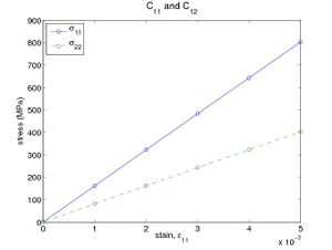
The above script ﬁrst generates a 3 × 3 × 3 perfect diamond cubic structure of Si. It then applies tensile strain in increments of 0.1% along [100] direction by the command shiftbox, and calculate the corresponding Virial stress at each strained state by the command eval. From the log ﬁle, the stress components $σ 11$ and $σ 22$ can be obtained and plotted as a function of the applied strain $ε 11$ . Fig. 1(a) plots the result from running the script with Stillinger-Weber(SW) potential. The slopes of these lines give $C 11 =$ 160.6 (GPa) and $C 12 =$ 80.5 (GPa).

To compute $C 44$ , which is the proportional constant between $σ 12$ and $ε 12$ , we can simply insert the following lines before quit in the above script.

incnfile = relaxed.cn readcn
input = [ 1 2 0.001 ] shiftbox relax eval
input = [ 1 2 0.001 ] shiftbox relax eval
input = [ 1 2 0.001 ] shiftbox relax eval
input = [ 1 2 0.001 ] shiftbox relax eval
input = [ 1 2 0.001 ] shiftbox relax eval

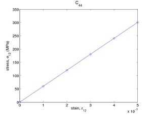
These commands shear the crystal in increments of $ε 12 =$ 0.1%. Again, from the log ﬁle, the stress component $σ 12$ can be obtained and plotted as a function of the applied strain. The result from SW potential is plotted in Fig. 1(b), from which we obtain $C 44 =$ 60.2(GPa). The values for C11 , C12 , and C44 obtained here are consistent with the original paper.<ref>H. Balamane, T. Halicioglu, and W. A. Tiler, PRB 46 2250-2279</ref>

Fig.1
(a)
(b)

Using the potential energy

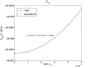
Sometimes, the simulation code does not implement the Virial stress calculation. In ab initio simulations, the Virial stress is usually not very accurate. In these cases, we can compute the elastic constants by monitoring the potential energy of the system, because the strain energy density $W$ is defined as

$W = \frac{1}{2}\sigma_{ij}\epsilon_{ij} = \frac{1}{2}\epsilon_{ij} C_{ijkl} \epsilon_{kl}$ .

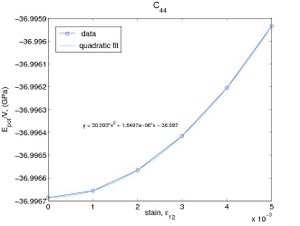
If the only nonzero strain is $ε 11$ , then the strain energy per volume becomes $W = C 11 ε 2 / 2$ . We can determine $C 11$ by ﬁtting $W (ε 11)$ to a parabola as shown in Fig.2(a). The elastic constnat $C 44$ can be determined in a similar way as shown in Fig.2(b). The elastic constants obtained in this way are $C 11 =$ 160.5(GPa) and $C 44 =$ 60.2(GPa), which are almost the same as the results obtained by using Virial stress.

The elastic constant $C 12$ is easily determined by the elastic relation

$B = \frac{1}{3}(C_{11} + 2C_{12})$

where $B$ is the bulk modulus, which we have already calculated in the manual 03. Since the bulk modulus of silicon is 108.3 (GPa) with SW potential, the elastic constant $C 12$ is

$C_{12} = \frac{1}{2}(3B - C_{11}) = 82.2$ (GPa)

Fig.2
(a)
(b)

Finding shear elastic constant for a non-tilting simulation cell

In the above sections, we compute $C 44$ by shearing the simulation cell. The simulation cell was rectangular before the shear, but becomes tilted after the shear. However, sometimes a simulation code allows to use only a rectangular simulation box and we can not tilt the box at all. In this case, how can we ﬁnd the shear elastic constant $C 44$ ? Notice that $C 11$ and $C 12$ can be always obtained with a rectangular cell, when the repeat vectors of the cell are aligned with the cubic axes of the crystal. With $C 11$ and $C 12$ C12 known, we can determine $C 44$ using the orthogonal transformation rule for the 4th order tensor. When the repeat vectors are not aligned with the cubic axes, we should be able to compute linear combination of $C 11$ , $C 12$ and $C 44$ while keeping the simulation cell rectangular. Remember that $C 11$ , $C 12$ and $C 44$ are components of a 4th order tensor which transforms as

C i j k l = T m i T n j T s k T t l C m n s t

where $T_{ij} = \mathbf{e}_i \cdot \mathbf{e}'_j$ is relation between two coordinate systems { $\mathbf{e}_i$ } and { $\mathbf{e}'_j$ }.

For example, if we have one coordinate system $\mathbf{e}_1$ = [1 0 0], $\mathbf{e}_2$ = [0 1 0] and $\mathbf{e}_3$ = [0 0 1], and another coordinate system $\mathbf{e}'_1$ = [1 1 0]/ \sqrt{2}, $\mathbf{e}'_2$ = [−1 1 0]/ \sqrt{2} and $\mathbf{e}'_3$ = [0 0 1], then the matrix [T] is

$[T] = \begin{pmatrix} 1/\sqrt{2} & -1/\sqrt{2} & 0 \\ 1/\sqrt{2} & 1/\sqrt{2} & 0 \\ 0 & 0 & 1 \end{pmatrix}$

In particular,

$\begin{align} C_{1111} &= T_{m1} T_{n1} T_{s1} T_{t1} C_{mnst} \\ &= \sum_{i=1}^3 T_{i1} T_{i1} T_{i1} T_{i1} C_{11} \\ & + 2(T_{11}T_{11}T_{21}T_{21} + T_{11}T_{11}T_{31}T_{31} + T_{21}T_{21}T_{31}T_{31})C_{12} \\ & + 4(T_{21}T_{31}T_{21}T_{31} + T_{11}T_{31}T_{11}T_{31} + T_{11}T_{21}T_{11}T_{21})C_{44}. \end{align}$

Suppose we create a perfect crystal such that x, y, and z axes of the simulation cell are aligned with $\mathbf{e}'_1$ , $\mathbf{e}'_2$ and $\mathbf{e}'_3$ . Then by straining the crystal along x axis, we can obtain <maht>C'_{1111}</math> = 180.4 (GPa) using the SW potential. Given $C 11$ = 160.6, $C 12$ = 80.5, the matlab script below gives $C 44$ = 59.9(GPa) for silicon.

% With given C11, C12, and C1111’, find C44 in cubic materials.
% C11, C12, and C44 are the elastic constants in Cartesian
% coordinate system.
% C1111’ is the elastic constant in the new coordinate.

syms C11 C12 C44
C11n = 160.6; C12n = 80.5; C44n = 60.2;
C1111prime = 180.40;
xyz0 = [ 1 0 0; % original coordinate
         0 1 0;
         0 0 1 ];
xyz1 = [ 1 1 0; % new coordinate
        -1 1 0;
         0 0 1 ];
T = zeros(3,3);
for i=1:3
    for j=1:3
        T(i,j) = dot(xyz0(i,:),xyz1(j,:)/norm(xyz1(j,:)));
    end
end

p=1; q=1; r=1; s=1;
A = T(1,p)*T(1,q)*T(1,r)*T(1,s) + T(2,p)*T(2,q)*T(2,r)*T(2,s) + ...
                                  T(3,p)*T(3,q)*T(3,r)*T(3,s);
B = T(1,p)*T(1,q)*T(2,r)*T(2,s) + T(1,p)*T(1,q)*T(3,r)*T(3,s) + ...
                                  T(2,p)*T(2,q)*T(3,r)*T(3,s);
C = T(2,p)*T(3,q)*T(2,r)*T(3,s) + T(1,p)*T(3,q)*T(1,r)*T(3,s) + ...
                                  T(1,p)*T(2,q)*T(1,r)*T(2,s);
CC = A*C11 + 2*B*C12 + 4*C*C44;
cc = subs(CC, C11, C11n); cc = subs(cc, C12, C12n);

disp(sprintf(’C44 = %f’,double(solve(cc-C1111prime,C44))))

Tcl version of MD++ script

For those who want to reproduce my results, I upload the Tcl version of MD++ script and the matlab script.
si_elastconst.tcl

# -*-shell-script-*-
#*******************************************
# Definition of procedures
#*******************************************
proc initmd { } { 
#MD++ setnolog
 MD++ setoverwrite
 MD++ dirname = runs/si_elastconst
 MD++ NIC = 200 NNM = 200
}

proc makecrystal { } { MD++ {
#--------------------------------------------
# Create Perfect Lattice Configuration
  element0 = Si   latticeconst = 5.43095
  crystalstructure = diamond-cubic  
  makecrystal
}} 

proc relax_fixbox { } { MD++ {
# Conjugate-Gradient relaxation
conj_ftol = 1e-6 conj_itmax = 1000 conj_fevalmax = 1000
conj_fixbox = 1  relax
} }

#*******************************************
# Main program starts here
#*******************************************
if { $argc == 0 } {
 set status 0
} elseif { $argc > 0 } {
 set status [lindex $argv 0]
}
puts "status = $status"

if { $status == 0 } {
# calculate elastic constants C_{11}, C_{12} and C_{44}
  initmd 

  MD++ latticesize = \[ 1 0 0 5 0 1 0 5 0 0 1 5 \]
  makecrystal 

  MD++ saveH eval
  set vol0     [MD++_Get OMEGA]
  
  set fileID [open "C11_C12.dat" w]
  for {set i -10} {$i <= 10} {incr i} {    
    set strain [expr $i/10000.0]
    MD++ restoreH input = \[ 1 1 $strain \] changeH_keepS
    relax_fixbox
    MD++ eval
  
    set sigma11 [expr (-1)*[MD++_Get TSTRESSinMPa_xx]]
    set sigma22 [expr (-1)*[MD++_Get TSTRESSinMPa_yy]]
    set EPOT    [MD++_Get EPOT]

    puts $fileID "[format %18.14e $strain]\t \
                  [format %18.14e $sigma11]\t \
                  [format %18.14e $sigma22]\t \
                  [format %18.14e [expr $EPOT/$vol0]]"
  }
  close $fileID

  set fileID [open "C44.dat" w]
  for {set i -10} {$i <= 10} {incr i} {    
    set strain [expr $i/10000.0]
    MD++ restoreH input = \[ 1 2 $strain \] changeH_keepS
    relax_fixbox
    MD++ eval
  
    set sigma12 [expr (-1)*[MD++_Get TSTRESSinMPa_xy]]
    set EPOT    [MD++_Get EPOT]

    puts $fileID "[format %18.14e $strain]\t \
                  [format %18.14e $sigma12]\t \
                  [format %18.14e [expr $EPOT/$vol0]]"
  }
  close $fileID  
  MD++ quit
  
} elseif { $status == 1 } {
# calculate elastic constants C'_{1111} in different coordinate
  initmd 

  MD++ latticesize = \[ 1 1 0 5 -1 1 0 5 0 0 1 7 \]
  makecrystal
  MD++ saveH eval
  set vol0     [MD++_Get OMEGA]
  
  set fileID [open "C1111prime.dat" w]
  for {set i -10} {$i <= 10} {incr i} {    
    set strain [expr $i/10000.0]
    MD++ restoreH input = \[ 1 1 $strain \] changeH_keepS
    relax_fixbox
    MD++ eval
  
    set sigma1111 [expr (-1)*[MD++_Get TSTRESSinMPa_xx]]
    set EPOT    [MD++_Get EPOT]
    
    puts $fileID "[format %18.14e $strain]\t \
                  [format %18.14e $sigma1111]\t \
                  [format %18.14e [expr $EPOT/$vol0]]"
  }
  close $fileID
  MD++ quit
  
} else {

  puts "unknown status = $status"
  MD++ quit
}

% Matlab script to calculate the elastic constants C11, C12 and C44
% of DC Si
clear, clf

B = 108.3e3;         % Bulk modulus of Si (in MPa) obtained from M02
data = load('C11_C12.dat');
strain11 = data(:,1);
sigma11 = data(:,2); % stress component sigma_{11} in MPa
sigma22 = data(:,3); % stress component sigma_{22} in MPa
Wn = data(:,4);       % strain energy density in eV/A^3

data = load('C44.dat');
strain12 = data(:,1);
sigma12 = data(:,2);
Ws = data(:,3);

if(exist('C1111prime.dat','file'))
    data = load('C1111prime.dat');
    strain1111 = data(:,1);
    sigma1111 = data(:,2);
    W1111 = data(:,3);
end
%%%%%%%%%%%%%%%%%%%%%%%%%%%%%%%%%%%%%%%%%%%%%%%%%
% plot the lattice energy vs lattice constant
% and find the equilibrium lattice constant, a_0
[P, S] = polyfit(strain11,sigma11,1);
C11 = P(1);
[P, S] = polyfit(strain11,sigma22,1);
C12 = P(1);
[P, S] = polyfit(strain11,Wn,2);
C11_e = P(1)*160.2e3*2;   
[P, S] = polyfit(strain12,sigma12,1);
C44 = P(1);
[P, S] = polyfit(strain12,Ws,2);
C44_e = P(1)*160.2e3*2; 
if(exist('C1111prime.dat','file'))
    [P, S] = polyfit(strain1111,sigma1111,1);
    C1111 = P(1);
    [P, S] = polyfit(strain1111,W1111,2);
    C1111_e = P(1)*160.2e3*2;    
end

disp(sprintf('-----------------------------------------------------'))
disp(sprintf('From Virial stress calculation,'))
disp(sprintf(['the elastic constants C11 = %10.8e, C12 = %10.8e, ',...
             'C44 = %10.8e in MPa.'],C11,C12,C44))
disp(sprintf('Then bulk modulus B = (C11 + 2*C12)/3 = %10.8e in MPa.',(C11+2*C12)/3))         
disp(sprintf('-----------------------------------------------------'))
disp(sprintf('From energy calculation,'))
disp(sprintf('the elastic constants C11 = %10.8e, C44 = %10.8ein MPa.',...
             C11_e, C44_e))
disp(sprintf('Then C12 = (3*B - C11)/2 = %10.8e in MPa', (3*B - C11_e)/2))
disp(sprintf('-----------------------------------------------------'))
if(exist('C1111prime.dat','file'))
disp(sprintf('-----------------------------------------------------'))
disp(sprintf('In e1=[1 1 0], e2=[-1 1 0] and e3=[0 0 1] coordinate, '))
disp(sprintf('the elastic constants C1111 = %10.8e (MPa) from stress calculation',C1111))
disp(sprintf('                      C1111 = %10.8e (MPa) from energy calcualtion',C1111_e))
disp(sprintf('-----------------------------------------------------'))
end

figure(1)
set(gca,'fontsize',14)
plot(strain11, sigma11, '.-',strain11, sigma22,'.-r',...
     strain12, sigma12, '.-g'), grid
xlabel('Strain','fontsize',16), 
ylabel('Stress (MPa)','fontsize',16)
legend('\epsilon_{11} vs. \sigma_{11}','\epsilon_{11} vs. \sigma_{22}',...
       '\epsilon_{12} vs. \sigma_{12}',2)

figure(2)
set(gca,'fontsize',14)
plot(strain11, Wn, '.-', strain12, Ws, '.-r'), grid
xlabel('Strain','fontsize',16), 
ylabel('Strain Energy Density, \it W \rm (eV/Angstrom^3)','fontsize',16)
legend('\epsilon_{11}','\epsilon_{12}',2)

Notes

Manual 07 for MD++ Computing Elastic Constants