Manual 02 for MD++
Making a Perfect Crystal

Nov 25 , 2007

---

Many solid materials have a periodic crystal structure.<ref>Glass is a counter-example, which is noncrystalline. We call it an amorphous material. Sometimes people consider it as supercooled liquid instead of a true solid, because, like a liquid, glass can flow under shear stress, although at very slow rate.</ref> For example, copper and aluminum have the face-centered-cubic (FCC) structure, while molybdenum and tungsten have the body-centered-cubic (BCC) structure under ambient conditions. The periodic arrangement of atoms simplifies the process of setting up an atomistic simulation, because we can use a periodic array of atoms as the initial condition. Thus, building up a crystal structure is often the first step in the atomistic simulation of solids. In this manual, we will learn how to build several crystal structures in MD++ with the example scripts.

---

Contents 1 Face-centered-cubic crystal 2 Body-centered-cubic crystal 3 Diamond-cubic crystal 4 Hexagonal-close-packed (HCP) structure 5 Zinc Sulphide (ZnS) 6 Notes

Face-centered-cubic crystal

First, let's make a perfect FCC aluminum crystal. The script file al.script, together with other script files discussed in this manual, can be found in the directory MD++/scripts/ME346. To run this script file, type

$ cd ~/Codes/MD++
$ bin/md_gpp scripts/ME346/al.script

The executable file, md_gpp does not contain any potential model, but can be used to visualize the atomic structure, as mentioned in the Manual 01.<ref>You can compile the executable alglue_gpp, which is a glue potential model for aluminum by typing

$ make alglue build=R.</ref> 

Here is the content of the al.script file.

# -*-shell-script-*-
setnolog
setoverwrite
dirname = runs/al-example     # To specify run directory

#--------------------------------------------
# Create Perfect Lattice Configuration
crystalstructure = face-centered-cubic
latticeconst = 4.05           # lattice constant for Al (unit: Angstrom)
latticesize = [ 1 0 0 1       # c1 = 1*[1 0 0] periodicity vec. in x
                0 1 0 1       # c2 = 1*[0 1 0] periodicity vec. in y
                0 0 1 1]      # c3 = 1*[0 0 1] periodicity vec. in z
makecrystal

#-------------------------------------------------------------
# Plot Configuration
atomradius = 1.0 bondradius = 0.3 bondlength = 0
atomcolor = blue highlightcolor = purple backgroundcolor = gray
bondcolor = red fixatomcolor = yellow
plotfreq = 10 win_width = 600 win_height = 600
rotateangles = [ 0 0 0 1.0 ]
openwin alloccolors rotate saverot eval plot
sleep quit

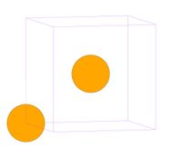
• Fig.1 Visualization of FCC structure
• 

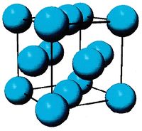
  (a) Conventional image of FCC unit cell

• 

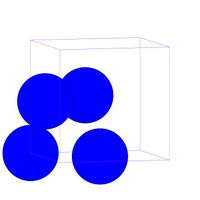
  (b) FCC unit cell in MD++. One corner atom and three face-centered atoms per cell

• 

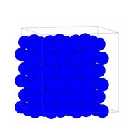
  (c) FCC of 3X3X3 cells

FCC, as well as HCP (Hexagonal Close Packed), is a close-packed crystal structure. In Fig.1(a), you can see the conventional image of FCC unit cell structure, where there is an atom at every corner and every face center of the cube. Since each corner atom is shared by 8 adjacent cubes and each face-centered atom is shared by 2 cubes, the total number of atoms per unit cell will be . In MD++, four atoms will be plotted per unti cell as shown in Fig.1(b), which is exactly what you see when you run al.script. Now imagine that the unit cell is replicated periodically in all 3 directions to fill the entire space. This would create an infinitely large crystal. We can create a larger crystal by modifying the latticesize variable, e.g.

latticesize = [ 1 0 0 3
                0 1 0 3
                0 0 1 3]

This creates a crystal with unit cells as shown in the Fig.1(c). The plot section of this script file will be explained in Manual 06.

Ex. 1 Make a perfect crystal of copper (Cu) of 4 X 4 X 4 unit cells. Cu has an FCC crystal structure and its equilibrium lattice constant is a = 3.6030 Å. You can use md_gpp as the executable file<ref>For MD simulations of Cu or Al, the fourth column of latticesize should not be smaller than 4 due to the relatively large cut-off radius in their potential models (eam or alglue).</ref> if you only want to visualize the structure. Use eam_gpp if you would like to do some computation using the potential model. (For example, the eval command computes the total potential energy of the structure.) For the latter case, you need to insert the following two lines into your script file after dirname.

potfile = ~/Codes/MD++/potentials/EAMDATA/eamdata.Cu
eamgrid = 5000 readeam

This reads the data needed by the EAM potential model of Cu.

Ex. 2 Make a perfect crystal of argon (Ar) of 4 X 4 X 4 unit cells. Ar is inert gas at room temperature but its solid state is face-centered-cubic crystal below its melting temperature T_m = 83.81K. Ar can be simulated by the Leonard-Jones potential model or the executable lj_gpp. Modify scripts/ME346/ar.script and run it by typing

$ bin/lj_gpp scripts/ME346/ar.script

---

Body-centered-cubic crystal

The BCC structure has an atom at every corner and body-center of each cube (unit cell), as shown in Fig.2(a). Molybdenum (Mo) is one example of BCC materials. Run mo.script file by typing

$ bin/fs_gpp scripts/ME346/mo.script

Here is the content of the mo.script file.

# -*-shell-script-*-
setnolog
setoverwrite
dirname = runs/mo-example

#--------------------------------------------
# Read the potential file
potfile = ~/Codes/MD++/potentials/mo_pot readpot

#--------------------------------------------
# Create Perfect Lattice Configuration
crystalstructure = body-centered-cubic
latticeconst = 3.1472         # in Angstrom for Mo
latticesize = [ 1 0 0 3
                0 1 0 3
                0 0 1 3 ]
makecrystal finalcnfile = perf.cn writecn

#---------------------------------------------
# Plot Configuration
atomradius = 1.0 bondradius = 0.3 bondlength = 0
atomcolor = orange highlightcolor = purple backgroundcolor = gray
bondcolor = red fixatomcolor = yellow
plotfreq = 10 win_width = 600 win_height = 600
rotateangles = [ 0 0 0 1 ]
openwin alloccolors rotate saverot eval plot
sleep quit

• Fig.2 Visualization of BCC structure
• 

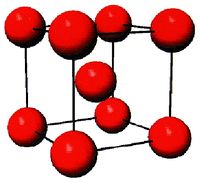
  (a) Conventional image of BCC unit cell

• 

  (b) BCC unit cell in MD++. One corner atom and one body-centered atom per cell

• 

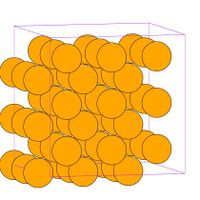
  (c) BCC of 3X3X3 cells

In the Fig.2(c), the simulation box (i.e. supercell) is defined by three periodicity vectors, , and : The command makecrystal generates the perfect crystal of molybdenum based on the given variables, crystalstructure<ref>Other possible values for crystalstructure are “simple-cubic”, “face-centered-cubic”,“L1_2”, “L1_0”, “diamond-cubic”, “zinc-blende”, etc. For a complete list, please read src/lattice.h.</ref> , latticeconst, and latticesize. The configuration will be saved as perf.cn in the directory of runs/mo-example by the command writecn. The configuration file contains the number of atoms and the position of all the atoms in terms of scaled coordinates followed by a 3 X 3 matrix, , whose columns are the three periodicity vectors, , and . The real coordinates of an atom, is related to the scaled coordinates through matrix multiplication

.

where a is the lattice constant.

Ex. 3 Make a perfect crystal of tantalum (Ta) with repeat vectors . Ta has a BCC lattice structure with an equilibrium lattice constant a = 3.3058 Å. Read the FS potential file for Ta by inserting the following line in the script.

potfile = ~/Codes/MD++/potentials/ta_pot readpot

---

Diamond-cubic crystal

Silicon (Si) has diamond-cubic structure, which can be regarded as two FCC structures offset by [1 1 1]/4. You can run the example script si.script by typing

 $ bin/sw_gpp scripts/ME346/si.script

where the executable sw_gpp contains the SW potential model for Si. The visualization window will look like Fig.3(b). Here is the content of the si.script file.

# -*-shell-script-*-
setnolog
setoverwrite
dirname = runs/si-example

#------------------------------------------------------------
#Create Perfect Lattice Configuration
#
crystalstructure = diamond-cubic
latticeconst = 5.43095            # (in Angstrom) for Si
latticesize = [ 1 0 0 2
                0 1 0 2
                0 0 1 2 ]
makecrystal writecn

#------------------------------------------------------------
#Plot Configuration
#
atomradius = 0.67 bondradius = 0.3 bondlength = 2.8285 
atomcolor = orange highlightcolor = purple
bondcolor = red backgroundcolor = gray70
plotfreq = 10 rotateangles = [ 0 0 0 1.25 ]
openwin alloccolors rotate saverot eval plot
sleep quit

• Fig.3 Visualization of DC structure
• 

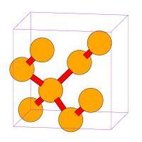
  (a) DC unit cell in MD++. 8 atoms per cell

• 

  (c) DC of 2X2X2 cells

Hexagonal-close-packed (HCP) structure

Conventionally, an HCP structure has repeated hexagonal or parallelogram cells (red line in Fig. 4(a)), neither of which satisfies periodic boundary conditions imposed along three orthogonal axes (x, y, and z). So, in MD++ we use a rectangular unit cell (blue line in Fig.4(a)), which contains 4 atoms as shown in Fig.4 (b). The scaled coordinates of these 4 atoms are (0,0,0), (0.5, 0.5, 0), (0.5, 1/6, 0.5) and (0, 2/3, 0.5) in the rectangular unit cell.

The script hcp-mg.tcl, shown below, creates HCP structure. Note that MD++ variable latticeconst now takes three values. The 1st one is the lattice constant a, and the last one is the lattice constant c. The 2nd argument can be ignored. For HCP, c is mostly a * sqrt(8/3) = 1.633 a. You can assign the c/a ratio somewhat different from 1.633.

 $ bin/md_gpp scripts/Examples/hcp-mg.tcl

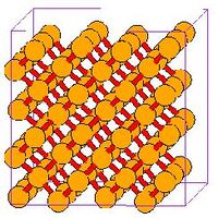
• Fig.4 HCP structure
• 

  (a) HCP conventional unit cell (red) and HCP rectangular unit cell (blue) (b) HCP unit cell in MD++. 4 atoms per cell

• 

  (c) HCP structure of 6X4X4 cells

# -*-shell-script-*-
# HCP structure
MD++ setnolog
MD++ setoverwrite
MD++ dirname = runs/HCP
#------------------------------------------------------------
#Create Perfect Lattice Configuration
#
set latt0 3.184
set c_over_a 1.633
MD++ latticestructure = hexagonal-ortho
# x-axis: [1 0 0] = [-1 2 -1 0]/3, 
# y-axis: [0 1 0] = [1 0 -1 0], 
# z-axis: [0 0 1] = [0 0 0 1] c-axis
MD++ latticesize = \[ 1 0 0 6 \
                      0 1 0 4 \
                      0 0 1 4 \]  
MD++ latticeconst = \[$latt0 0.0 [expr $latt0*${c_over_a}] \]
MD++ makecrystal 
MD++ element0 = Mg atommass = 24.305 # g/mol
MD++ makecrystal finalcnfile = perf.cn writecn
#------------------------------------------------------------
#Plot Configuration
#
MD++ {
atomradius = [1.3] #bondradius = 0.3 bondlength = 0
atomcolor0 = yellow atomcolor1 = "light grey"
highlightcolor = purple  bondcolor = red backgroundcolor = gray
fixatomcolor = yellow
plot_atom_info = 1
plotfreq = 10
rotateangles = [ 0 0 0 1.2 ]
openwin alloccolors rotate saverot refreshnnlist eval plot
}
MD++ sleep quit

Zinc Sulphide (ZnS)

ZnS is a two component material and has two lattice structures (zinc-blende and Wurtzite). Through the following example script, we will learn how to use MD++ to generate multi-component material in zinc-blende strucutre or Wurtzite structure.

 $ bin/md_gpp scripts/Examples/example06a-ZnS.script

Here is the content of the example06a-ZnS.script file, which will creat a Zinc-blende structure of ZnS.

# -*-shell-script-*-
# Zincblende structure of ZnS
setnolog
setoverwrite
dirname = runs/ZnS-example
#------------------------------------------------------------
#Create Perfect Lattice Configuration
#
latticestructure = zinc-blende
element0 = Zn element1 = S atommass = [65.409 32.065] # g/mol
latticeconst = 5.42           #(A) 
latticesize = [ 1  0  0  2    #(x)
                0  1  0  2    #(y)
                0  0  1  2  ] #(z)
makecrystal finalcnfile = perf.cn writecn
#------------------------------------------------------------
#Plot Configuration
#
atomradius = [1.3 1] #bondradius = 0.3 bondlength = 2.8285
atomcolor0 = "light grey" atomcolor1 = yellow
highlightcolor = purple  bondcolor = red backgroundcolor = gray
fixatomcolor = yellow
plot_atom_info = 1
plotfreq = 10
rotateangles = [ 0 0 0 1.2 ]
openwin alloccolors rotate saverot refreshnnlist eval plot
sleep quit

Similarly, you can create a Wurtzite structure by the following script, example06b-ZnS.script.

# -*-shell-script-*-
# Wurtzite structure of ZnS
# (screw dislocation motion under fixed boundary)
setnolog
setoverwrite
dirname = runs/ZnS-example
#------------------------------------------------------------
#Create Perfect Lattice Configuration
#
latticestructure = wurtzite
element0 = Zn element1 = S atommass = [65.409 32.065] # g/mol
latticeconst = [3.82 0 6.24]  #(in Angstrom)
latticesize = [ 1  0  0  2    #(x)
                0  1  0  2    #(y)
                0  0  1  2  ] #(z)
makecrystal finalcnfile = perf.cn writecn
#------------------------------------------------------------
#Plot Configuration
#
atomradius = [0.8 1] bondradius = 0.3 bondlength = 3.25
atomcolor0 = "light grey" atomcolor1 = yellow
highlightcolor = purple  bondcolor = red backgroundcolor = gray
fixatomcolor = yellow
plot_atom_info = 1
plotfreq = 10
rotateangles = [ 0 0 0 1.2 ]
openwin alloccolors rotate saverot refreshnnlist eval plot
sleep quit

• Fig.5 ZnS structure
• 

  (a) Zinc-blende structure of ZnS

• 

  (c) Wurtzite structure of ZnS

Notes

<references/>