Revision as of 16:07, 22 December 2007

Manual 09 for MD++
Computing Ideal Strength

Keonwook Kang and Wei Cai

Dec 8 , 2007

Ideal strength is the theoretical limit up to which a defect-free material can sustain external load before it breaks. We define ideal strength as the maximum derivative of the excess energy (per area) that comes from rigid translation of part of material.<ref>There is different definition of ideal strength. Roudy and Cohen calculated it from the excess energy of uniform deformation of material.(D. Roudy and M. L. Cohen, Phys. Rev. B 64 212103 (2001))</ref> In this manual, it is explained how the ideal strengths of diamond cubic structure of Si are calculated with MD++ codes. This task was part of work covered in our paper<ref name=kangcai2007>Keonwook Kang and Wei Cai, Philosophical Magazine, 87 2169–2189 (2007)</ref>.

Ideal Tensile Strength

Let’s assume that we want to calculate the ideal tensile strength $\sigma_{[110]}^{\mathrm{th}}$ along the [1 1 0] direction of Si. First, a simulation cell is created with the three periodicity vectors $\mathbf{c}_1 = N_x [1 1 0]$ , $\mathbf{c}_2 = N_y[\bar{1} 1 0]$ and $\mathbf{c}_3 = N_z[0 0 1]$ , each of which is aligned along $x$ , $y$ and $z$ direction, respectively. Make sure that the cell is subjected to periodic boundary condition (PBC) in all three directions. Next, the potential energy change is recorded as the function of the opening distance $d$ when the (1 1 0) surface opens rigidly (See Fig. 1(a).) or

γ = γ(d)

.

where $γ$ is the excess energy to create two free surfaces. In order to rigidly separate a bulk crystal, we could collectively translate half of atoms but instead we used a simple trick. When we redefine the periodicity vector $\mathbf{c}_1$ as

$\mathbf{c}_1 = \left( 1 + \frac{d}{L_x^0}\right) \mathbf{c}_1^0$ .

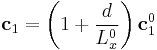while fixing the coordinates of all the atoms, it gives the same effect of separating the bulk crystal into two by $d$ . We change the box length $L_x \equiv a|\mathbf{c}_1|$ by redefining the periodicity vector $\mathbf{c}_1$ from its initial definition $\mathbf{c}^0_1$ with certain ratio and it will create a gap of width $d$ in $x$ direction between the periodic image (2) and the crystal (1) in the primary cell as shown in Fig. 1(a).

In MD++ Codes, there is a command changeH_keepR which changes one of periodicity vectors with atoms fixed. The input to this command has three numbers.

input = [ i j frac ] changeH_keepR

The first number is the index of the periodicity vector that you want to change. For example, if i=1, $\mathbf{c}_1$ vector will be changed. (2 for $\mathbf{c}_2$ and 3 for $\mathbf{c}_3$ ) The second number is the index of direction. If j=1, the fraction frac of the vector $\mathbf{c}_1$ is added to itself and $\mathbf{c}_1$ can be longer or shorter depending on the sign of frac. If j=2, the vector $\mathbf{c}_1$ will be tilted by the fraction frac of $\mathbf{c}_2$ vector.

Do not forget to refresh the neighbor list whenever you change $\mathbf{H}\equiv [\mathbf{c}_1\, \mathbf{c}_2\, \mathbf{c}_3]$ while atoms’ positions are fixed. MD++ automatically refreshes the neighbor list based on the change of the atoms’ positions. If atoms are fixed, the list will not be updated even if there could be a virtual displacement of atoms by changing $\mathbf{H}$ . In the script (given at the end of this manual), you will see the command clearR0, right after changeH_keepR, which enforces the neighbor list to be refreshed. There are more MD++ commands to be explained: saveH stores the current 3×3 matrix H to H0 and restoreH restores H from H0. RHtoS converts the real coordinate $\mathbf{r}_i$ of an atom $i$ to the scaled coordinate $\mathbf{s}_i$ by $\mathbf{s}_i = \mathbf{H}^{-1} \mathbf{r}_i$ .

If we plot $γ$ vs. $d$ , the curve looks like Fig. 2(a). As $d$ increases, the energy also increases up to a plateau $2γ s$ , where $γ s$ is the (unrelaxed) surface energy of (1 1 0) plane of Si. Once the opening distance becomes longer than certain cutoff distance, the interaction between two parts no longer plays a role and the energy becomes constant and irrelative to $d$ . You may be aware that the slope of the $γ(d)$ curve has the unit of stress. We define the maximum value of the slope as the ideal tensile strength along the separation direction, e.g. [1 1 0]. The SW potential model gives $\sigma_{[110]}^{\mathrm{th}}$ =41.7 (GPa) for Si.

Fig.1
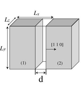
(a) Separating a bulk crystal across a (1 1 0) plane by distance $d$ .
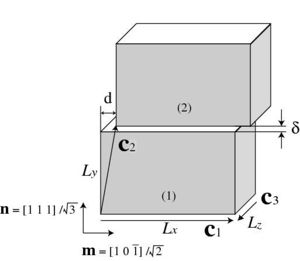
(b) The generalized stacking fault energy for slip on a (1 1 1) plane can be computed by tilting the repeat vector $\mathbf{c}_2$ of the simulation cell while keeping the position of all atoms fixed. These figures are excerpted from our paper.<ref name="kangcai2007"/>

Ideal Shear Strength

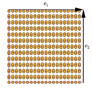
The procedure of calculating ideal shear strength is pretty much similar to that for ideal tensile strength except that we now have to deal with 2-dimensional array of energy. In Fig. 1(b), it is illustrated how we slip part of a bulk crystal to the rest. For example, the periodicity vectors are chosen to be $\mathbf{c}_1 = N_x[1 0 \bar{1}]$ , $\mathbf{c}_2 = N_y[1 1 1]$ and $\mathbf{c}_3 = N_z[1 \bar{2} 1]$ to calculate the ideal shear strength $\sigma^{\mathrm{th}}_{(111)[10\bar{1}]}$ . The simulation cell is subject to PBC in all three directions. With the coordinates of all the atoms fixed, redefining $\mathbf{c}_2$ vector as

$\begin{align} \mathbf{c}_2 &= \left(1+ \frac{\delta}{L_z^0}\mathbf{c}_2^0 + \frac{d}{L_x^0}\mathbf{c}_1^0 \right) \\ &= (L_z^0 + \delta)\mathbf{n} + d\mathbf{m} \end{align}$

makes $\mathbf{c}_2$ vector tilted and as a result the periodic image (2) will be shifted and moved from the crystal (1) in the primary cell by $d$ and $δ$ , respectively. Notice that we do not simply slip but also allow the crystal move normal to slip plane and the energy $γ$ is a function of $d$ and $δ$ or

γ = γ(d,δ)

.

Because the crystal will in reality adjust the gap $δ$ to reach energy-minimum state for a given slipped distance $d$ , what we really want is $min δ (d)$ and denote it as $Γ$ or

$\Gamma = \displaystyle\min_{\{\delta\} }\gamma ( d )$ .

The curve $Γ(d)$ is shown in Fig. 2(b). The shifted distance $d$ is normalized by the magnitude of Burgers vector and we observe that the misfit energy is periodic after one Burgers vector. The ideal shear strength is also defined as the maximum slope of the misfit energy curve and it is 9.5 GPa from SW potential model.

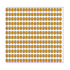
You have to keep it in mind that the shuffle set plane of (1 1 1) is your slip plane. Fig. 3 shows two configurations which would be same unless you tilt the periodicity vector. After the vector $\mathbf{c}_2$ is tilted, one gives $Γ$ of shuffle-set plane and the other gives that of glide-set plane. And the ideal shear strength of glide-set plane (e.g. 77.3GPa from SW) is much higher than that of shuffle-set plane. In MD++ script, this is handled by the command pbcshiftatom, which shifts whole atoms periodically by dx, dy, and dz in all three directions.

input = [dx dy dz] pbcshiftatom

The numbers dx, dy and dz are given in scaled coordinate.

In MD++, there is a command calmisfit calculating the misfit energy $γ$ as $d$ and $δ$ change.

 input = [ surfacenormal
           x0 dx x1
           y0 dy y1
           z0 dz z1 ]
 calmisfit

The input variable needs seven elements, the first of which indicates the surface normal index. If it is 2, the slip plane normal is in $y$ -direction (1 for $x$ and 3 for $z$ -direction) and the periodicity vector $\mathbf{c}_2$ is going to be tilted. The rest six numbers are basically grid points to designate to which direction and how much the periodicity vector is tilted (or stretched). The numbers are normalized by the length of one lattice vector in each direction. If dx=0.001, the increment of tilting the vector in $x$ -direction would be $0.001 \times a \times |\mathbf{c}_1|/N_x$ , where $a$ is the lattice constant. If dy=0.01, the vector $\mathbf{c}_2$ increases by the amount of 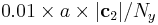$0.01 \times a \times |\mathbf{c}_2|/N_y$ in $y$ direction. In our example, the last three numbers are all zeros or z0 = dz = z1 = 0.

After running calmisfit, a text file “Emisfit.out” will be dumped out and it will be used to calculate the ideal shear strength by the Matlab script attached at the end.

Fig.2
(a) The excess energy per area is plotted as a function of the opening
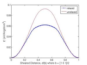
(b) Misfit energy $Γ$ vs. the shifted distance $d$ . SW potential model is used for atomistic simulation in (a) and (b).

Fig.3
(a)
(b) Two configurations in (a) and (b) are essentially identical before the periodicity vector $\mathbf{c}_2$ is tilted. After $\mathbf{c}_2$ is tilted along $\mathbf{c}_1$ direction, the crystal is shifted on glide-set plane in (a) and shuffle-set plane in (b).

Ideal Shear Strength in Non-tilting Cell

Sometimes we simply cannot tilt the periodicity vectors. For example, the original Baskes’ MEAM codes are implemented only for a rectangular cell. In this case, the procedures explained above can not be applied and we have to move a chunk of atoms literally. Fig. 4(a) shows the initial configuration in which a few layers at top and bottom are removed in order to have room for atoms to be shifted as shown in Fig. 4(b). Other than that, the rest of process to get the ideal shear strength is identical.

To remove top and bottom atoms, two MD++ commands fixatoms_by_position and removefixedatoms are used. The command fixatoms_by_position fixes atoms within a hexahedral volume defined by six numbers (x0, x1, y0, y1, z0 and z1 in scaled coordinate) in input

input = [enable x0 x1 y0 y1 z0 z1 ] fixatoms_by_position

when enable=1. Then the command removefixedatoms removes those fixed atoms.

MD++ codes have another command calmisfit2 to calculate the misfit energy in non-tilting cell. The input variable for calmisfit2 has six more numbers (xmin, xmax, ymin, ymax, zmin and zmax) than calmisfit to define a hexahedral volume which will be moved by the command. Those numbers should be given in scaled coordinate.

 input = [ surfacenormal
           x0 dx x1
           y0 dy y1
           z0 dz z1
           xmin xmax ymin ymax zmin zmax]
 calmisfit2

The command calmisfit2 also produces a text file, “Emisfit.out” of the same format and the same Matlab script will read it to calculate the ideal shear strength.

Fig.4
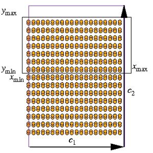
(a) Configuration to calculate the ideal shear strength in non-tilting simulation cell: (a) the initial configuration and (b) the shifted configuration
(b)

Script

The MD++ script and the Matlab script are given below for those who want to reproduce the results or try to calculate the ideal strength of other crystal materials. Let’s say MD++ script file name is “idealstr.tcl”. If you type

$ bin/sw_gpp scripts/work/idealstr.tcl 0

it calculates the surface energy of (1 1 0) plane in terms of the opening distance $d$ . If you type

$ bin/sw_gpp scripts/work/idealstr.tcl 1

it calculates the misfit energy of (1 1 1) plane along $[1\, 0\, \bar{1}]$ direction by tilting the periodicity vector $\mathbf{c}_2$ . If you type

$ bin/sw_gpp scripts/work/idealstr.tcl 2

it will calculate the same misfit energy in different method explained in Sec. 3.

MD++ Script

# -*-shell-script-*-
source "scripts/Examples/Tcl/startup.tcl"
#*******************************************
# Definition of procedures
#*******************************************
proc initmd { } {
  MD++ setnolog
  MD++ setoverwrite
  MD++ dirname = runs/si_idealstr
  MD++ NIC = 200 NNM = 200
}

proc openwindow { } { MD++ {
# Plot Configuration
  atomradius = 0.67 bondradius = 0.3 bondlength = 0
  atomcolor = orange bondcolor = red backgroundcolor = gray70
  win_width = 300 win_height = 300
  plotfreq = 10 rotateangles = [ 0 0 0 1.25 ]
  plot_atom_info = 1 # reduced coordinates of atoms
#  plot_atom_info = 2 # real coordinates of atoms
#  plot_atom_info = 3 # energy of atoms
openwin alloccolors rotate saverot eval plot
} }

#*******************************************
# Main program starts here
#*******************************************
if { $argc == 0 } {
  set status 0
} elseif { $argc > 0 } {
  set status [lindex $argv 0]
}

puts "status = $status"

if { $status == 0 } {
# calculate surface opening energy on (1 1 0).
  initmd
  MD++ {
    element0 = Si latticeconst = 5.43095
    crystalstructure = diamond-cubic
    latticesize = [ 1 1 0 5
                   -1 1 0 5
                    0 0 1 7 ]
    makecrystal }
  MD++ saveH eval
  set Lx0 [MD++_Get H_11]
  set Ly0 [MD++_Get H_22]
  set Lz0 [MD++_Get H_33]
  set EPOT0 [MD++_Get EPOT]
  set Area [expr $Ly0 * $Lz0]
  set fileID [open "Esurf.dat" w]
  for {set i -10} {$i <= 100} {incr i} {
    set strain [expr $i/1000.0]
    MD++ restoreH RHtoS
    MD++ input = \[ 1 1 $strain \] changeH_keepR
    MD++ clearR0 # enforce refresh neighbor list
    MD++ eval
    set Lx [MD++_Get H_11]
    set dist [expr $Lx - $Lx0]
    set EPOT [MD++_Get EPOT]
    # Esurf2 : excessive energy per area to create 2 free surfaces.
    set Esurf2 [expr ($EPOT - $EPOT0)/$Area]
    puts $fileID "[format %18.14e $dist]\t \
                  [format %18.14e $Esurf2]"
  }
  close $fileID
  MD++ quit

} elseif { $status == 1 } {
# calculate generalized stacking fault energy on (1 1 1) along [1 0 -1]
  initmd
# surface normal direction 1/x 2/y 3/z
  set surfacenormal 2
  set lattconst 5.43095
  set c1 "1 0 -1"; set c2 "1 1 1"; set c3 "1 -2 1"
  set Nx 5; set Ny 4; set Nz 3

  set gridx " 0.000 0.005 0.500"
  set gridy "-0.050 0.010 0.150"
  set gridz " 0.000 0.050 0.000"

# write the matlab script
  set fileID [open "parameter.m" w]
  puts $fileID "normaldir = $surfacenormal"
  puts $fileID "latticeconst = $lattconst"
  puts $fileID "latticesize = \[ $c1 $Nx "
  puts $fileID "                 $c2 $Ny "
  puts $fileID "                 $c3 $Nz \]"
  puts $fileID "dxyz = \[ $gridx "
  puts $fileID "          $gridy "
  puts $fileID "          $gridz \]"
  close $fileID

  MD++ {
    element0 = Si
    crystalstructure = diamond-cubic
  }
  MD++ latticeconst = $lattconst
  MD++ latticesize = \[$c1 $Nx $c2 $Ny $c3 $Nz\]
  MD++ makecrystal

# To make shuffle set of (111) plane exposed
  MD++ { input = [0 0.05 0 ] pbcshiftatom }
  MD++ input = \[ $surfacenormal $gridx $gridy $gridz \]
  MD++ calmisfit
  MD++ quit

} elseif { $status == 2 } {
# calculate generalized stacking fault energy on (1 1 1) along [1 0 -1]
  initmd
# surface normal direction 1/x 2/y 3/z
  set surfacenormal 2
  set lattconst 5.431
  set c1 "1 0 -1"; set c2 "1 1 1"; set c3 "1 -2 1"
  set Nx 5; set Ny 6; set Nz 3
  set gridx " 0.000 0.005 0.500"
  set gridy "-0.050 0.010 0.150"
  set gridz " 0.000 0.050 0.000"
  set xmin -1.00; set xmax 1.00
  set ymin  0.01; set ymax 1.00
  set zmin -1.00; set zmax 1.00

# write the matlab script
  set fileID [open "parameter.m" w]
  puts $fileID "normaldir = $surfacenormal"
  puts $fileID "latticeconst = $lattconst"
  puts $fileID "latticesize = \[ $c1 $Nx "
  puts $fileID "                 $c2 $Ny "
  puts $fileID "                 $c3 $Nz \]"
  puts $fileID "dxyz = \[ $gridx "
  puts $fileID "          $gridy "
  puts $fileID "          $gridz \]"
  close $fileID

  MD++ {
    element0 = Si
    crystalstructure = diamond-cubic
  }
  MD++ latticeconst = $lattconst
  MD++ latticesize = \[$c1 $Nx $c2 $Ny $c3 $Nz\]
  MD++ makecrystal

  MD++ input = \[1 -1 1 0.4 1 -1 1 \] fixatoms_by_position removefixedatoms
  MD++ input = \[1 -1 1 -1 -0.42 -1 1 \] fixatoms_by_position removefixedatoms
  MD++ input = \[ $surfacenormal $gridx $gridy $gridz $xmin $xmax $ymin $ymax $zmin $zmax \]
  MD++ calmisfit2

  openwindow
  MD++ sleep quit
  MD++ quit

} else {
puts "unknown status = $status"
MD++ quit
}

Matlab Script

After running MD++, you just run the following matlab script in the directory where the output files exist. Then the matlab script will plot the energy curve and calculate ideal strengths.

%#! /usr/local/bin/octave -qf
% Matlab script, cal_idealstr.m
% to calculate ideal tensile strength "sigma" and shear strength "tau"
clear

%%%%%%%%%%%%%%%%%%%%%%%%%%%%%%%%%%%%%%%%%%%%%%%%%%%%%%%%%
% calculate ideal tensile strength along [110] direction
%%%%%%%%%%%%%%%%%%%%%%%%%%%%%%%%%%%%%%%%%%%%%%%%%%%%%%%%%
data = load(’Esurf.dat’);
d = data(:,1);     % openning distance in A
gamma = data(:,2); % excessive energy per area creating 2 free surfaces (eV/A^2)

sigma = max(gamma(2:end)-gamma(1:end-1))/(d(2) - d(1)) * 160.2;
disp(sprintf(’Ideal tensile stregnth = %e(GPa)’,sigma));

figure(1)
set(gca,’fontsize’,14)
plot(d, gamma, ’.-’), grid
xlabel(’Opening Distance \it d \rm(Angstrom)’,’fontsize’,16),
ylabel(’\gamma (eV/Angstrom^2)’,’fontsize’,16)
line([-1 1.1],[gamma(end) gamma(end)],’linewidth’,2,’color’,’k’)
text(-1.3, gamma(end),’2\gamma_s’,’fontsize’,16)

%%%%%%%%%%%%%%%%%%%%%%%%%%%%%%%%%%%%%%%%%%%%%%%%%%%%%%%%%%%%%%%%
% calculate ideal shear strength on (111) along [110] direction
%%%%%%%%%%%%%%%%%%%%%%%%%%%%%%%%%%%%%%%%%%%%%%%%%%%%%%%%%%%%%%%%
if (~exist(’parameter.m’,’file’))
    error(’No parameter.m found’)
else
    parameter

    dx = dxyz(1,2); dy = dxyz(2,2); dz = dxyz(3,2);
    vx = latticesize(1,1:3); Lx = latticeconst*norm(vx);
    vy = latticesize(2,1:3); Ly = latticeconst*norm(vy);
    vz = latticesize(3,1:3); Lz = latticeconst*norm(vz);

    data = load(’Emisfit.out’);
    Mx=max(data(:,1)); My=max(data(:,2)); Mz=max(data(:,3));

%%%%%%%%%%%%%%%%%%%%%%%%%%%%%%%%%%%%
% convert data to relaxed energy
    MM=-sort(-[Mx+1,My+1,Mz+1]);         % Then MM(1) > MM(2) > MM(3)
    E = reshape(data(:,4),MM(1),MM(2));

    Erlx = zeros(MM(1),1);
    Zrlx = zeros(MM(1),1);

    normalgrid = dxyz(normaldir,1):dxyz(normaldir,2):dxyz(normaldir,3);
    normalfinegrid = dxyz(normaldir,1):dxyz(normaldir,2)/1000:dxyz(normaldir,3);

    for i = 1:MM(1),
        a = E(i,:);
        a_interp = interp1(normalgrid,a,normalfinegrid,’spline’);
        [Erlx(i), ind] = min(a_interp);
        Zrlx(i) = normalfinegrid(ind);
    end

% retrieve unrelaxed energy
    Eunrlx=E(:,find(abs(normalgrid)<1e-8));

% calculate ideal shear strength
    tau = max(Erlx(2:end)-Erlx(1:end-1))/(dx*Lx) * 160.2;
    disp(sprintf(’Ideal shear stregnth = %e(GPa)’,tau));

    figure(2); set(gca,’fontsize’,14)
    plot([0:Mx]/Mx, Erlx-Erlx(1), ’b.-’,...
         [0:Mx]/Mx, Eunrlx-Eunrlx(1),’r-’);
    legend(’relaxed’,’unrelaxed’);
    xlabel(’Sheared Distance, d/|b| where b = [1 0 1]/2’,’fontsize’,16)
    ylabel(’\Gamma (eV/Angstrom^2)’,’fontsize’,16)

    figure(3); set(gca,’fontsize’,14)
    plot([0:Mx]/Mx,Zrlx, ’r.-’, ...
         [0 1],[1 1]*dxyz(normaldir,1),’b-’,...
         [0 1],[1 1]*dxyz(normaldir,3),’b-’);
    xlabel(’Sheared Distance, d/|b| where b = [1 0 1]/2’,’fontsize’,16)
    ylabel({’Lowest energy height,’; ’\delta/|c_2| where c_2 = [1 1 1]’},’fontsize’,16)
end

Notes