Revision as of 15:36, 13 April 2008

Manual 05 for MD++
Molecular Dynamics Simulations

Keonwook Kang and Wei Cai

[First written, [ Jan 19 ]], 2007

[Last Modified, [ Mar 03 ]], 2008

The case studies described in Manuals 02-04 only deal with atomic positions as degrees of freedom. For example, in Manual 02, we learned how to create a perfect crystal by MD++ command makecrystal. In Manual 03, we varied the size of the perfect crystal to find the equilibrium lattice constants. In Manual 04, we introduced a vacancy to the perfect crystal and let the atomic positions relax to a local energy minimum. In this manual, we will learn how to perform finite temperature, Molecular Dynamics (MD) simulations. For this purpose, we will need to deal with atomic velocities as degrees of freedom, as well as a number of control variables, such as integrator type, time step, and output controls. We will learn to specify the simulation ensembles from different choices: microcanonical (NVE), canonical (NVT), isoenthalpic-isobaric (NPH) and constant pressure/temperature (NPT) ensembles. Different quantities are conserved or controlled in different ensembles. For example, the total number of atoms (N), volume (V) and energy (E) are conserved in the (NVE) ensemble.

The NVE ensemble is the probably the best starting point to understand what happens in MD simulations. In Statistical Mechanics, to picture the NVE ensemble, we can imagine a system of N gas molecules inside a rigid container with perfect thermal insulation. Hence no work or heat can be exchanged between the system and the outside world (its environment). While the gas molecules move with time, the total number of particles N, the total energy E and the total volume V of the system does not change. A large number of replicas of the system with the same N, V, E forms the NVE, or microcanonical ensemble in Statistical Mechanics. In MD simulations within the NVE ensemble, we usually do not simulate the rigid container --- this is because the simulation volume is usually very small and having an explicit container will lead to a large surface-to-volume ratio and large simulation artifacts. Instead, periodic boundary conditions (PBC) are usually used in MD simulation. If the repeat vectors of PBC do not change, the simulation volume V is kept constant during the simulation. Since the particles follows Hamiltonian dynamics in MD simulations, the total energy E is conserved. The total number of particles N is obviously conserved in the MD simulation. Therefore, MD simulations under PBC with fixed repeat vectors and no thermostats (to be described later) correspond to the NVE (microcanonical) ensemble.

The following input script mo_NVE.tcl gives an example of running MD simulations in MD++. You can test is by the following command (if you put this file in your scripts/ directory)

$ bin/fs_gpp scripts/mo_NVE.tcl

This example script first creates a perfect BCC crystal of molybdenum (Mo) with a supercell of 5[1 0 0] $\times$ 5[0 1 0] $\times$ 5[0 0 1]. It then runs MD simulations using the Finnis-Sinclair (FS) potential.

# -*-shell-script -*-
# run NVE MD simulation of perfect crystal of Mo.
#
#*******************************************
# Definition of procedures
#*******************************************
proc initmd { } { MD++ {
#setnolog
setoverwrite
dirname = runs/mo-example
zipfiles = 1   # zip output files
#
#--------------------------------------------
# Create Perfect Crystal
element0 = Mo
crystalstructure = body-centered-cubic
latticeconst = 3.1472           # in Angstrom for Mo
latticesize = [ 1 0 0 5
                0 1 0 5
                0 0 1 5]
}}
#------------------------------------------------------------
proc readMoPot { } { MD++ {
# Read the potential file
potfile = ~/Codes/MD++/potentials/mo_pot readpot
}}
#-------------------------------------------------------------
proc openwindow { } { MD++ {
# Plot Configuration
atomradius = 1.0 bondradius = 0.3 bondlength = 2.725
atomcolor = orange highlightcolor = purple
bondcolor = red backgroundcolor = gray70
plotfreq = 10 rotateangles = [ 0 0 0 1.25 ]
openwin alloccolors rotate saverot eval plot
}}
#--------------------------------------------
proc setup_md { } { MD++ {
#MD settings
ensemble_type = "NVE" integrator_type = "VVerlet"
T_OBJ = 300        # (in Kelvin) Desired Temperature
atommass = 95.94   # (in g/mol)
timestep = 0.001   # (in ps)
totalsteps = 2000
# save property every 10 steps
saveprop = 1 savepropfreq = 10
savecn = 0   savecnfreq = 100
writeall = 1 DOUBLE_T = 1 
randseed = 12345 srand48 #randomize random number generator

#*******************************************
# Main program starts here
#*******************************************
initmd
readMoPot
MD++ makecrystal finalcnfile = perf.cn writecn
openwindow
#---------------------------------------------
# run MD
setup_md
MD++ initvelocity finalcnfile = init.cn writecn
#format of thermodynamic property file
MD++ {output_fmt = "curstep EPOT KATOM Tinst"}
MD++ outpropfile = thermo.out openpropfile
MD++ run closepropfile
MD++ finalcnfile = 300K-5X5X5.cn writecn eval
MD++ sleep quit
}}

In this Tcl script, we start with some definition of functions that will be used subsequently. The main program starts after the comment Main program starts here. The program first calls the initmd function that was defined at the beginning, which opens the output directory. After creating the perfect crystal using the makecrystal command, it calls the setup_md function that initializes some important parameters for MD simulation. (Commands and variables related with visualization as specified in the openwindow function will be covered in a separate manual in detail.)

The first line in the setup_md function selects the statistica ensemble for the simulation. The possible choices for the variable ensemble_type are NVE, NVT, NPH and NPT. The type of the numerical integrator is specified by the integrator_type variable and can be either the Gear 6-th order predictor-corrector algorithm (Gear6) or the velocity Verlet algorithm (VVerlet). The predictor-corrector integrator has a higher order of accuracy but velocity Verlet is a symplectic integrator and is more stable at larger algorithm. We recommend the use of velocity Verlet algorithm whenever possible (i.e. if it is implemented for the chosen ensemble type).

The variable atommass specifies the atomic mass in unit of g/mol. timestep specifies the integrator time step $Δ t$ in unit of picosecond. totalsteps is the total number of time steps for the MD simulation. Hence totalsteps times timestep is the total time duration of the MD simulation. We usually choose timestep to be as large as possible provided that the total energy of the system is conserved within an acceptable accurady. totalsteps is usually chosen so that the total simulation time is long enough for the system to reach an equilibrium or steady state (usually on the order of picoseconds).

The command initvelocity assign random numbers to the atomic velocities and then scale them so that the instantaneous temperature matches the target value, as specified by T_OBJ in unit of K. Strictly speaking, temperature is not well defined in an NVE ensemble (but is well defined in the NVT ensemble). Here we can regard T_OBJ as a measure of the instantaneous kinetic energy of the system. MD++ uses the drand48() to generate random numbers for the velocities. The random number generator can be initialized by calling srand48 with a specified randseed. This approach is more convenient for debugging because the same randseed garauntees exactly the same random number sequence will be generated if you run the simulation again. On the other hand, you may use the function srandbytime to use the current time as the random seed for initializing the random number generator. This makes sure that ever time you run the simulation again a completely different set of random numbers will be generated.

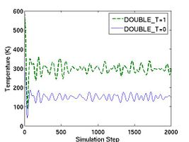
If the parameter DOUBLE_T is set to 1, then the velocities are scaled in such a way that the instantaneous temperature is twice of T_OBJ, as illustrated in Fig.1. The reason we may want to set DOUBLE_T = 1 is the following. When we assign velocities to the atoms in a perfect crystal, the instantaneous temperature almost always drop to half of its initial value when thermal equilibrium is reached (see Fig.1). This is due to the energy equipartition theorem. For solids at temperatures much below the melting temperature, the Hamiltonian is close to that of a set of coupled harmonic oscillators. The total energy of a harmonic system is equally divided between the average kinetic energy and the average potential energy. Because the total energy is conserved in an NVE-ensemble simulation, the kinetic energy is bound to decrease by half if the kinetic energy and potential energy (initially zero) are equal (in time average) when equilibrium is reached. Setting DOUBLE_T = 1 allows the temperature at the equilibrium state to match the desired temperature.

Fig.1 Instantaneous temperature as a function of time during MD simulations with different settings for DOUBLE_T.

The parameters saveprop and savepropfreq specify whether or not and how often the simulation properties will be saved periodically in a data file. If saveprop = 1 and savepropfreq = 10, the properties such as potential energy, kinetic energy and temperature will be save every 10 simulation steps, provided that the MD++ command openpropfile is called before the command run. The name of the property file is specified by the outputfile variable and is prop.out by default. The setting zipfiles = 1 at the beginning of this script file (line 11) specifies that both property files and atomic configuration files (see below) will be automatically zipped (by gzip) after they are written.

The content of a property ﬁle is defined by variable output_fmt. In this example, each line of the property file will contain the current step (curstep), potential energy (EPOT), kinetic energy (KATOM), and temperature (Tinst). If we do not specify output_fmt, the default content of the property file will be current step (curstep), kinetic energy (KATOM), potential energy (EPOT), pressure (PRESSURE), $σ x y$ (TSTRESS_xy), $σ y z$ (TSTRESS_yz), $σ z x$ (TSTRESS_zx), HELM, the extended energy(HELMP), thermodynamic friction coeﬃcient (zeta), reversible work increment dEdlambda and volume (OMEGA). The energies are in unit of eV and stresses in eV/A˚^3. Please note that there is an overall minus sign between the stress variables in MD++ and that in conventional elasticity theory. For example, a positive pressure correspond to positive normal stress components in MD++ but negative normal stress components in elasticity theory. This is because in MD++, we followed the sign convention of Parrinello and Rahman for stress control.<ref>M. Parrinello and A. Rahman, "Polymorphic transitions in single crystals: A new molecular dynamics method", J. Appl. Phys 52 7182-7190 1981</ref>

The parameters savecn and savecnfreq specify whether or not and how often the atomic coordinates (and velocities if writeall = 1) will be saved as .cn files during the MD simulation. If savecn = 1 and savepropfreq = 10000, the intermediate .cn files will be saved every 10000 steps, provided that the MD++ command openintercnfile is called before the command run. The name of the intermediate .cn files are specified by the intercnfile variable and is inter####.cn by default, where #### are integers (starting with 0000) that will be automatically incremented by one after each file is written. In this example, savecn = 0 so no intermediate .cn files will be saved. After all the relevant parameters have been set up, the MD++ command run starts the MD simulation.

After the simulation is finished, a property file named thermo.out will be written in the output directory runs/mo-example. This file can be loaded and plotted by programs such as Matlab, Octave, or Gnuplot.<ref>A simple way to plot the total energy using gnuplot (a free software on Unix/Linux) is to run the command.

plot "thermo.out" u ($1):($2+$3) with line

</ref> Fig.2 plots the total energy per atom and instantanous temperature for two simulations with different sizes. The larger system (10[100] $\times$ 10[010] $\times$ 10[001]) has eight times more atoms than the smaller one (5[100] $\times$ 5[010] $\times$ 5[001]). As expected, the data for the larger system experience less statistical fluctuation.

Fig.2 Energy and Temperature fluctuation of NVE ensemble
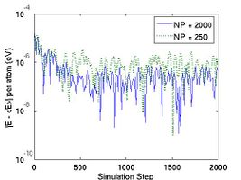
(a) Energy Fluctuation in NVE ensemble.
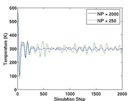
(b) Temperature in NVE ensemble

After the run command, the script file calls the command writecn to save the final atomic configuration into a .cn file whose name is specified by finalcnfile. The .cn file has the following format. The first line contains the total number of atoms NP. The following NP lines then contain the scaled coordinates of all atoms: $s_x^{(i)}$ , $s_y^{(i)}$ , $s_z^{(i)}$ , $i = 1, 2, \cdots NP$ . The last three lines of the .cn file specify a 3 $\times$ 3 matrix $\mathbf{H}$ whose column vectors are the three repeat vectors of the simulation supercell (subjected to periodic boundary conditions). The real coordinates of an atom (x, y, z ) and the scaled coordinates for each atom are related through $\mathbf{H}$ as follows

$\left( \begin{array}{c} x \\ y \\ z \end{array} \right) = \left( \begin{array}{ccc} H_{11} & H_{12} & H_{13} \\ H_{21} & H_{22} & H_{23} \\ H_{31} & H_{32} & H_{33} \end{array} \right) \left( \begin{array}{c} s_x \\ s_y \\ s_z \end{array} \right)$ .

If writeall = 1 is specified before writecn, additional informations are added to the NP lines of data. Following the scaled coordinates, each line will also contain the scaled velocities (_VSR[i].x, _VSR[i].y and _VSR[i].z), local potential energy (_EPOT_IND[i]), flag (fixed[i]), central-symmetry-deviation paramter (_TOPOL[i]), atom species (species[i]), atom groups (group[i]) and image index (image[i]). You can see this diﬀerence by comparing two conﬁguration ﬁles, perf.cn (written before setting writeall = 1) and init.cn (written after). If writevelocity = 1 is used instead of writeall = 1, then only the scaled velocities are added behind the three columns for scaled coordinates.

At the end of the example script, the command sleep is called so that the graphics window to stay open (i.e. alive) for a while so that we can examine the atomic structure. You can press ctrl-c in the terminal to exit. You can also comment out the sleep command in the script file so that MD++ exits immediately after reaching the end of the input file.

Canonical(NVT) Ensemble

The following example script mo_NVT.tcl reads the structure file of BCC Mo and runs NVT MD simulation during which temperature is maintained at 300 K using Nose-Hoover thermostat<ref> S. Nose, “A Molecular Dynamics Method for Simulations in the Canonical Ensemble”, Molecular Physics, 52 255 (1984)</ref>. Run the script by typing

$ bin/fs_gpp scripts/mo_NVT.tcl

# -*-shell-script -*-
# run NVT MD simulation of perfect crystal of Mo.
#
#*******************************************
# Definition of procedures
#*******************************************
proc initmd { } { 
         ...
}
#------------------------------------------------------------
proc readMoPot { } { 
         ...
}
#-------------------------------------------------------------
proc openwindow { } { 
         ...
}
#--------------------------------------------
proc setup_md { } { MD++ {
#MD settings
ensemble_type = "NVT" integrator_type = "VVerlet"
implementation_type = 0 vt2 = 1e28
T_OBJ = 300       # (in Kelvin) Desired Temperature
atommass = 95.94  # (g/mol)
timestep = 0.001 # (ps)
totalsteps = 2000
saveprop = 1 savepropfreq = 10
savecn = 0 savecnfreq = 100
writeall = 1
}}
#*******************************************
# Main program starts here
#*******************************************
initmd
readMoPot
MD++ {
  incnfile = 300K-5X5X5.cn
  atommass = 95.94 timestep = 0.001
  readcn eval
}
openwindow
#---------------------------------------------
# run MD
setup_md
MD++ {output_fmt = "curstep EPOT KATOM Tinst HELMP"}
MD++ outpropfile = thermo-NVT.out openpropfile
MD++ run eval 
#reverse velocity (to test reversibility)
MD++ input = -1 multiplyvelocity
#MD simulation (reverse)
MD++ run eval
MD++ finalcnfile = 300K-5X5X5-NVT.cn writecn
MD++ sleep quit

Instead of creating BCC Mo crystal, this script reads the conﬁguration ﬁle 300K_5X5X5.cn, which was generated by the previous script mo_NVE.tcl, using the MD++ command readcn. Note that when MD++ reads the configuration ﬁle, the timestep should be idnetical with that of the previous run because the scaled velocity is stored as dimensionless unit after being multiplied with the timestep. It is safe that you specify timestep and atommass when reading .cn ﬁle as shown in the script.

Setting ensemble_type = "NVT" activates Nose-Hoover thermostat, which basically adds an additional variable ( $ζ$ ) to the system such that the temperature is controlled by the feedback routine virtually mimicking heat transfer to the heat reservoir,

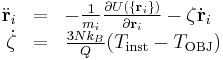$\begin{array}{rcl} \ddot\mathbf{r}_i &=& -\frac{1}{m_i}\frac{\partial U(\{\mathbf{r}_i\})}{\partial \mathbf{r}_i} - \zeta \dot\mathbf{r}_i \\ \dot\zeta &=& \frac{3N k_B}{Q} ( T_{\mathrm{inst}} - T_{\mathrm{OBJ}} ) \end{array}$ .

when the degree of freedom is 3N. In MD++, Nose-Hoover thermostat are implemented in three diﬀerent way, each of which uses different integrator deﬁned through implementation_type. If it is zero, the implicit integrator will be chosen. If it is one, the explicit integrator based on Sto¨rmer-Verlet method will work. If it is two, another explicit integrator based on Liouville formulation will be activated.

Thermal coeﬃcient vt2 is related with thermal mass Q of Nose´-Hoover thermostat as

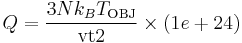$Q = \frac{3 N k_B T_{\mathrm{OBJ}}}{\mathrm{vt2}}\times (1e+24)$ .

where N is number of atoms and k_B is the Boltzmann constant (8.617343e-5 eV/K). For convenience, we also defined thermal mass NHMass, which is exactly Nose'-Hoover thermal mass Q. When N = 250 and T = 300 K (or k_B T ~ 0.026 eV), vt2 = 1e28 corresponds to NHMass = 1.95e-03. The bigger vt2 is (or the smaller NHMass is), the faster the response of the system is to control the temperature. The eﬀect of vt2 on Helmholtz free energy and temperature ﬂuctuation is shown in Fig. 3.

Fig.3 The Effect of Nose-Hoover Mass in NVT MD
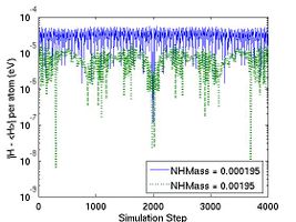
(a) Helmholtz energy fluctuation in NVT ensemble.
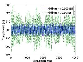
(b) Temperature in NVT ensemble

HELMP in the output_fmt is Helmholtz free energy which is the conserved quantity in NVT MD.

multiplyvelocity multiplies the number speciﬁed by the preceding input to all velocity components of all atoms. With input=-1, the MD++ command multiplyvelocity reverses the velocity direction of all the atoms and they are expected to be at the initial position after the reverse run. This is done to test the reversibility of the symplectic integrator. Comparing two configuration files 300K-5X5X5.cn and 300K-5X5X5-NVT.cn reveals that the numbers become different after 10^(-14) digit. If we consider the total step is 4000, the difference at each step would be O(10^(-17)), which corresponds to the machine precision. On the other hand, if you test integrator_type = Gear6, the numbers become different only after 10^(-6) digit. We can say the symplectic integrator is indeed reversible.

Canonical(NVT) Ensemble with Nose-Hoover Chain

Martyna et al<ref>G. J. Martyna, M. L. Klein and M. Tuckerman, "Nose-Hoover chains: The canonical ensemble via continuous dynamics", J. Chem. Phys. 97 2635--2643</ref> modified the original Nose-Hoover thermostat such that a chain of thermostats is added instead of one thermostat. The purpose of this chain method is to increase the size of the phase space and help the system to be ergodic even when the system is stiff or its dynamics is not ergodic. To implement the Nose-Hoover chain integrator, we refered another paper of Martyna's.<ref>G. J. Martyna, "Explicit reversible integrators for extended systems dynamics", Molecular Physics 87 1117-1157 (1996)</ref>

The MD++ script Mo_NVTC.tcl, given below, shows how to run Nose-Hoover chain method in MD++ to obtain a system of canonical ensemble.

# -*-shell-script -*-
# run NVE MD simulation of perfect crystal of Mo.
#
#*******************************************
# Definition of procedures
#*******************************************
proc initmd { } { MD++ {
    ....
}}
#------------------------------------------------------------
proc readMoPot { } { MD++ {
    ....
}}
#-------------------------------------------------------------
proc openwindow { } { MD++ {
    ....
}}
#--------------------------------------------
proc setup_md { } { MD++ {
#MD settings
ensemble_type = "NVTC" integrator_type = "VVerlet"
NHChainLen = 4                       # MAXNHCLEN = 20 in md.h
NHMass = [ 1.95e-4 2e-6 2e-6 2e-6 ]
T_OBJ = 300        # (in Kelvin) Desired Temperature
atommass = 95.94   # (in g/mol)
timestep = 0.001   # (in ps)
totalsteps = 5000
saveprop = 1 savepropfreq = 10
savecn = 0 savecnfreq = 100
writeall = 1
DOUBLE_T = 0 randseed = 12345 srand48
}}

#*******************************************
# Main program starts here
#*******************************************
initmd
readMoPot
MD++ {
  incnfile = ../mo-example/300K-5X5X5.cn
  atommass = 95.94 timestep = 0.001
  readcn eval
}
openwindow
#---------------------------------------------
# run MD
setup_md
MD++ {output_fmt = "curstep EPOT KATOM Tinst HELMP"}
MD++ outpropfile = thermo-NVTC.out openpropfile
MD++ run eval
MD++ sleep quit
}}

You choose the ensemble type to be NVTC. The number of chains and masses of each chain can be specified using NHChainLen and NHMass. According to my experience, NHMass needs to be chosen with caution, otherwise the system may lose its reversibility, even though Martyna et al stated that the choice of thermal mass NHMass is not critical. In fact, they also presented how to take reasonable choice of NHMass.

NHMass[0] ~  $N f k B T / ω 2$  where  is the number of degrees of freedom.
And NHMass[i] ~  $k B T / ω 2$  (for i = 2 to M, where M is the number of chains)

thermostat 1 to M -1 fluctuates at a frequency of omega.

Constant Stress (N $σ$ H) Ensemble

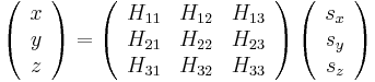
In constant stress ensemble, the stress is controlled to maintain the external stress (or the applied stress) using Parrinello-Rahman's method. The applied stress tensor $σ EXT$ can be decomposed as the sum of the hydrostatic term and the deviatoric term,

$\sigma_{\mathrm{EXT}} = \sigma_{\mathrm{EXT}}^{\mathrm{hydro}} + \sigma_{\mathrm{EXT}}^{\mathrm{devi}}$ .

where $\sigma_{\mathrm{EXT}}^{\mathrm{hydro}} = \frac{1}{3}(\sigma_{\mathrm{EXT}})_{kk}\cdot\mathrm{I}$ and $\sigma_{\mathrm{EXT}}^{\mathrm{devi}} = \sigma_{\mathrm{EXT}} - \sigma_{\mathrm{EXT}}^{\mathrm{hydro}}$ . Here we used the Einstein's convention, in which repeated indices are summed over from 1 to 3, to express the sum of the diagonal components of the stress tensor. Then the equations of motion of Parrinello-Rahman's method can be written as

$\begin{array}{rcl} \ddot\mathbf{r}_i &=& -\frac{1}{m_i}\frac{\partial U(\{\mathbf{r}_i\})}{\partial \mathbf{r}_i} - \mathbf{H}^{-T}\dot\mathbf{G}\mathbf{H}^{-1} \dot\mathbf{r}_i \\ \ddot\mathbf{H} &=& -\frac{1}{M} \left[ \left( \sigma_{\mathrm{Virial}} - \sigma_{\mathrm{EXT}}^{\mathrm{hydro}} \right)\Xi - \left( \mathbf{H}\mathbf{H}_0^{-1} \sigma_{\mathrm{EXT}}^{\mathrm{devi}} \right) \Xi_0 \right] \end{array}$ .

where $\mathbf{H}$ is the 3X3 box matrix at time t and $\mathbf{H}_0$ is the initial box matrix at t = 0. $\mathbf{G}$ is defined as $\mathbf{G} = \mathbf{H}^T\mathbf{H}$ and called the metric tensor. $\Xi = \Omega \mathbf{H}^{-T}$ and $\Xi_0 = \Omega_0 \mathbf{H}_0^{-T}$ are used to reduce the notation. ( $Ω$ is the volume of the box or $\Omega = \det{\mathbf{H}}$ .) M is the "box mass".

If we apply the constant pressure $P_{\mathrm{EXT}} = -\frac{1}{3}\left(\sigma_{\mathrm{EXT}}\right)_{kk}$ , the deviatoric part of the external stress is zero and the second equation becomes simply

$\ddot\mathbf{H} = -\frac{1}{M} \left[ \left( \sigma_{\mathrm{Virial}} + P_{\mathrm{EXT}}\mathbf{I} \right)\Xi \right]$ .

and this follows isoenthalpic-isobaric (NPH) Ensemble for large number of particles. The script Mo_NPH.tcl, given below, shows how we set parameters and commands to run NPH MD simulation using MD++.

# -*-shell-script -*-
# run NPH MD simulation of perfect crystal of Mo.
#
#*******************************************
# Definition of procedures
#*******************************************
proc initmd { } { MD++ {
        ...
}}
#------------------------------------------------------------
proc readMoPot { } { MD++ {
        ...
}}
#-------------------------------------------------------------
proc openwindow { } { MD++ {
        ...
}}
#--------------------------------------------
proc setup_md { } { MD++ {
#MD settings
ensemble_type = "NPH" integrator_type = "VVerlet"
wallmass = 1000 boxdamp = 0.1
saveH # Use current H as reference (H0), needed for specifying stress
stress = [ 1000    0    0
              0 1000    0
              0    0 1000 ] # compression in MPa
conj_fixboxvec = [ 0 1 1
                   1 0 1
                   1 1 0 ]
T_OBJ = 300                 # (in Kelvin) Desired Temperature
atommass = 95.94            # (in g/mol)
timestep = 0.001            # (in ps)
totalsteps = 10000
saveprop = 1 savepropfreq = 20
savecn = 0 savecnfreq = 100
writeall = 1
DOUBLE_T = 0 randseed = 12345 srand48
}}

#*******************************************
# Main program starts here
#*******************************************
initmd
readMoPot
MD++ makecrystal finalcnfile = perf.cn writecn
openwindow
#---------------------------------------------
# run MD
setup_md
MD++ initvelocity finalcnfile = init.cn writecn
MD++ {output_fmt = "curstep EPOT KATOM Tinst HELMP \
                    TSTRESSinMPa_xx TSTRESSinMPa_yy TSTRESSinMPa_zz \
                    TSTRESSinMPa_xy TSTRESSinMPa_xz TSTRESSinMPa_yz \
                    H_11 H_22 H_33 H_12 H_13 H_21 H_23 H_31 H_32" }
MD++ outpropfile = thermo-NPH.out openpropfile
MD++ run closepropfile
#MD++ finalcnfile = Mo-5X5X5-NPH.cn writecn eval
MD++ sleep quit
}}

First, you choose the ensemble type and the integrator type. wallmass corresponds to the box mass M of the Parrinello-Rahman (PR) method. boxdamp is used to make the system converge fast. You can see the effect of boxdamp in Fig.4. If boxdamp is nonzero, the box acceleration is redefined as

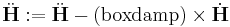
$\ddot\mathbf{H} := \ddot\mathbf{H}- (\mathrm{boxdamp}) \times \dot\mathbf{H}$

and the system becomes no longer symplectic. The external stress is assigned throuth MD++ variable stress in MPa. Note that the sign convention of stress is opposite of that from the elasticity theory. The positive stress in the MD++ script means that you apply compression to the system. conj_fixboxvec defines which component of the box matrix $H$ will be fixed. you need to specify $H 0$ by calling saveH before using the PR method. According to Ray and Rahman<ref>J. R. Ray and A. Rahman, "Statistical ensembles and molecular dynamics studies of anisotropic solids", J. Chem. Phys, 80 4423--4428 </ref>, " $H 0$ should be taken as the average value of $H$ when the stress is zero."

Fig.4 The Effect of Box Damp in NPH MD
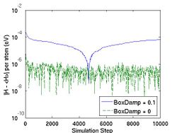
(a) Extended energy fluctuation in NPH ensemble.
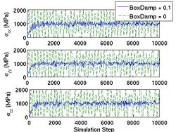
(b) Stress in NPH ensemble.
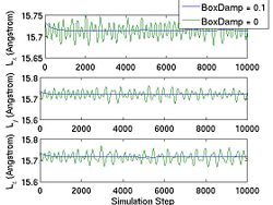
(c) Simulation box in NPH ensemble

Isothermal-isobaric (NPT) Ensemble

Revision as of 15:36, 13 April 2008

Manual 05 for MD++
Molecular Dynamics Simulations

Contents

Microcanonical (NVE) Ensemble

Canonical(NVT) Ensemble

Canonical(NVT) Ensemble with Nose-Hoover Chain

Constant Stress (N $σ$ H) Ensemble

Isothermal-isobaric (NPT) Ensemble

Revision as of 15:36, 13 April 2008

Manual 05 for MD++ Molecular Dynamics Simulations

Contents

Microcanonical (NVE) Ensemble

Canonical(NVT) Ensemble

Canonical(NVT) Ensemble with Nose-Hoover Chain

Constant Stress (NσH) Ensemble

Isothermal-isobaric (NPT) Ensemble

Manual 05 for MD++
Molecular Dynamics Simulations

Constant Stress (N $σ$ H) Ensemble