Manual 02 for ParaDiS
Straight dislocations in the Mo BCC metal

Dec. 14 , 2007

This manual is intended to explain how to create ParaDiS input files using a small fortran code called create_dislocations.f. It shows how to simulate a single dislocation, two dislocations and then several dislocations. Several parameters are introduced and explained.

Units in ParaDiS and DDLab

All units are in S.I. For instance, lengths are in meter, times in second, stresses in Pascal etc. There is a conversion factor that can be used in both ParaDiS and DDLab called burgMag. In BCC metals, the Burgers vector of a screw dislocation is of the type <111> so it is convenient to define parameters in units such that dislocations with Burgers vector <111> has a norm equals to one that is is on the form . burgMag is defined as burgMag = where a₀ is the lattice spacing. If the material is Molybdenum (Mo) then and burgMag = 2.710 ^{− 10}. In DDLab, burgMag is often set to one and in ParaDiS it is equals to by default. The default material in ParaDiS is molybdenum, defaults material constants are set to this material by default. In this manual, we use only the molybdenum material.

An infinitely long and straight dislocation

In this first example, we want to create a single dislocation under no applied stress and no loading conditions so that this dislocation is not moving during the simulation. The dislocation is chosen to be such that its Burgers vector is b = a₀ / 2[111] and its glide plane is . We choose a screw dislocation so its dislocation line is in the same direction as its Burgers vector.

We have created a small fortran file called create_dislocation.f. The input file is pretty simple, the user enters the length of the system in micrometers, the total number of steps, the name of the ParaDiS input file, the number of dislocations. Then for each dislocation, the user has to define its Burgers vector, its glide plane, its type and a random number seed.

An example of such an input file for a single dislocation is

10
300
one
1
1 1 1
1 -1 0
0
screw
478

In this simple example, we create a dislocation in a 10μm domain, we want to run the simulation for 300 time steps. The name of the ParaDiS input file is called one.cn and one.data. We have 1 dislocation, it has the Burgers vector [111] and the glide plane. It is a screw dislocation and the position of its dislocation line will be chosen at random. If the user wants to specify exactly the dislocation line, he/she can do it by replacing the three last lines by

1 300 300 300 -500 300 1000

In this case, the user defines the dislocation line by entering 6 numbers corresponding to a,b,c and x0,y0 and z0 in

x = a t+ x0 
y = b t+ y0 
z = c t+ z0

This input file will create a file called one.cn and one.data in the Runs directory as well as a one_result directory in the Outputs directory of ParaDiS.

It is important to note here that when one wants to create an infinite dislocation in bulk metal, one has to enforce the periodic boundary conditions or in other words the first point defining the dislocation line should touch one end of the simulation box and the last point of the dislocation line should be close to the simulation box but not touch it to respect periodic boundary conditions. The program create_dislocations.f does that automatically. Also it changes the values that the user enters to respect ParaDiS units and in particular uses burgMag.

Two infinitely long dislocations

Now we want to create two infinitely long dislocations. These dislocations are chosen to have Burgers vectors and b₂ = − b₁ and the same glide plane direction so that they attract each other and annihilate. The input file for [create_dislocation.f] is

3
1000
two
2
1 1 1
1 -1 0
1
0 0 1 0 0 0
-1 -1 -1
1 -1 0
1
0 0 1 1500 0 0

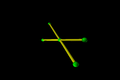
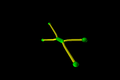
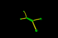
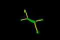
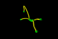
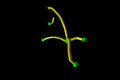
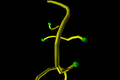
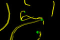
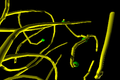
Initial configuration of these dislocations is shown in Fig 1[a]. These dislocations are distant of 1500 burgMag. A snapshot of the dynamics of these two dislocations is shown on Fig 1. First, the dislocations are attracted to each other (Fig 1[b-c]), and then the dislocations annihilate (Fig 1[d]).

• Figure 1: Two attracting dislocations
• 

  [a]

• 

  [b]

• 

  [c]

• 

  [d]

We now choose two dislocations with Burgers vectors with glide plane and with glide plane like in \cite{bulatov.etal}. These two dislocations are pinned at their extremities as shown in Fig. 3. We apply an uniaxial constant strain rate load of 1 per second. We can do that by setting the parameters

loadType = 1;
eRate = 1;
edotdir = [1 0 0];

in ParaDiS input file .cn. This loading condition favors dislocations multiplication and the stress-strain response of the material is shown in Fig.2.

Figure 2: Stress-strain response for two dislocations that are initially brought to intersection at their midpoints under constant strain rate loading with uniaxial loading direction [011].

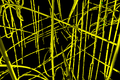
A snapshot of the simulation is shown in Fig. 3. We have used the povray output to generate these pictures. Some lines have to be added to ParaDiS input file to create povray outputs:

povray = 1 povrayfreq = 1 povraydt = -1.000000e+00 povraytime = 0.000000e+00 povraycounter = 1

• Figure 3: Snapshots of the simulation of two interacting dislocations. (a) Two dislocations are initially intersecting at their midpoints and are pinned at their extremities. (b)-(c) They form a zipping junction. (d)-(g) They unzip. (h)-(i) New dislocations are created and dislocations multiply.
• 

  [a]

• 

  [b]

• 

  [c]

• 

  [d]

• 

  [e]

• 

  [f]

• 

  [h]

• 

  [i]

• 

  [j]

Several straight dislocations

Now that we know how to use the code we are ready to do a simulation using a parallel computer. We set up 8 screw dislocations representative of BCC metals. We chose the following Burgers vectors and glide planes twice: b₁ = a₀ / 2[111], , , with respective glide planes: , , , . The position of the dislocations is chosen at random. We apply an uniaxial constant strain rate load of 1 per second. After a few thousand iterations on a one processor machine, the simulation output data start to slow down. We use the restart files to restart the simulation on a cluster using 16 processors. In order to do that we need to change the lines

numXdoms = 1
numYdoms = 1
numZdoms = 1

to

numXdoms = 2
numYdoms = 4
numZdoms = 2

When the simulation output data start to slow down again more processors are needed and we can increase the value of the above variables accordingly.

We choose the BCC_0 mobility law. It is defined by three parameters. MobEdge, MobScrew are the dislocation mobilities for the edge and screw component respectively and MobClimb is the edge dislocation climb mobility. The choice of these parameters is very important and will change dramatically the results of the simulation.

MobScrew =  0.1
MobEdge  =  0.55
MobClimb =  1/100

However in a real material, it is difficult for screw dislocations to climb. So we modified these parameters to account for that effect. The following parameters were used in \cite{bulatov.etal}, they correspond to a high effective temperature since the mobility of edges and screw are equal.

MobScrew =  10
MobEdge  =  10
MobClimb =  1/100000

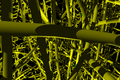
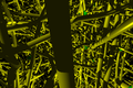
A snapshot of dislocation multiplication in this case is shown in Fig. 4. A comparison of both set of parameters is shown in Fig. 5 and Fig. 6. The second set gives rise to strain hardening whereas the first set does not. Also the size of the system chosen matters. If the system is too small (less than 5μm), no strain hardening will be observed.

• Figure 4: Snapshots of the simulation of eigth dislocations in the BCC Mo metal using the first set of paramters showing a higher and higher density of dislocations.
• 

  [a]

• 

  [b]

• 

  [c]

• 

  [d]

Figure 5: Comparison between two sets of parameters for the stress-strain response for eight screw dislocations under constant strain rate loading with uniaxial loading direction [100]. Plots are scaled for comparison.

Figure 6: Increase in the dislocation density in the case of eigth screw dislocations under constant strain rate loading with uniaxial loading direction [100]. Plots are scaled for comparison.