M04A Conjugate Gradient Method in MD++

Manual 04A for MD++
Conjugate Gradient Method in MD++

Keonwook Kang and Wei Cai

Mar 19 , 2009

---

Conjugate Gradient Method

The conjugate gradient (CG) method was initially proposed as an iterative method to solve a large linear system of equations, such as Failed to parse (SVG (MathML can be enabled via browser plugin): Invalid response ("Math extension cannot connect to Restbase.") from server "https://wikimedia.org/api/rest_v1/":): {\displaystyle \mathrm{A}\mathbf{x} = \mathbf{b}} , where A is an n by n symmetric (positive-definite) matrix, and b is an n by 1 vector. The basic idea is that the quadratic form of a function Ψ(x),

Failed to parse (SVG (MathML can be enabled via browser plugin): Invalid response ("Math extension cannot connect to Restbase.") from server "https://wikimedia.org/api/rest_v1/":): {\displaystyle \Psi(\mathbf{x}) = \frac{1}{2}\mathbf{x}^T \mathrm{A}\mathbf{x} - \mathbf{b}^T\mathbf{x} + c}

is minimized by the solution of Failed to parse (SVG (MathML can be enabled via browser plugin): Invalid response ("Math extension cannot connect to Restbase.") from server "https://wikimedia.org/api/rest_v1/":): {\displaystyle \mathrm{A}\mathbf{x} = \mathbf{b}} if A is symmetric and positive-definite. Later, Fletcher and Reeves adopted it to solve nonlinear optimization problems. In MD++, the CG method is used to find a meta-stable structure by minimizing a given (usu. nonlinear) potential energy function.

The algorithm of the CG method is structured by two nested loops. The outer loop tries different search directions, and the inner loop aims to find the optimal step length which minimizes the object function along a given search direction. The inner loop may not be needed when the exact expression of the optimal step length can be given. If a certain condition is met, the program exits out of the loops and stops. The algorithm is shown in figure 1.

Figure 1 Algorithm of the (nonlinear) CG method.

In figure 1, Ψ(x) is a function to be minimized, g is the gradient of Ψ, and s is the search direction. α_k is the optimal step length that minimizes the function Ψ(x_k+α_ks_k) at the k-th iteration. β_k+1 is the parameter related with update of the search direction.

Depending on how we choose β, the minimization methods can be different. For example, if β_k=0, it is the steepest descent (SD) method.

While there exists the analytical expression of α for a linear system, or

Failed to parse (SVG (MathML can be enabled via browser plugin): Invalid response ("Math extension cannot connect to Restbase.") from server "https://wikimedia.org/api/rest_v1/":): {\displaystyle \alpha_k=\Bigg\{}	${\frac {\mathbf {r} _{k}^{T}\mathbf {r} _{k}}{\mathbf {r} _{k}^{T}\mathrm {A} \mathbf {r} _{k}}}$	for SD,
	${\frac {\mathbf {r} _{k}^{T}\mathbf {r} _{k}}{\mathbf {s} _{k}^{T}\mathrm {A} \mathbf {s} _{k}}}$	for CG,

where r_k is the residual and is defined as $\mathbf {r} _{k}\equiv \mathbf {b} -\mathrm {A} \mathbf {x} _{k}$, for nonlinear problems, α is generally obtained by a numerical method such as Newton's method, quasi-Newton method, secant method, interpolation method, or other similiar methods. These methods of finding an optimal α are called as the line search methods. For details of the line search method, refer Nocedal and Wright's Numerial Optimization

For the CG method, the search directions are constructed by using the conjugacy of the residuals, or

$\mathbf {r} _{i}^{T}\mathbf {r} _{j}=0$      for      $i\neq j$.

From this condition, β_k is obtained as

$\beta _{k+1}\equiv {\frac {\mathbf {r} _{k+1}^{T}\mathbf {r} _{k+1}}{\mathbf {r} _{k}^{T}\mathbf {r} _{k}}}$.

For details of the derivation, refer J. R. Shewchuk's. The benefit of this choice is that a new search direction is orthogonal to all the previous search directions. In other words, we don't need to store all the previous search directions to produce a linearly independent new search direction.

Non-linear CG method

For non-linear CG method, there exist different choices of β as shown in table 1, in which the residual r_k is now defined as the negative gradient or $\mathbf {r} _{k}=-\mathbf {g} _{k}$.

Table 1. The update parameter β in non-linear CG. For more different choices of β, refer Hager and Zhang's.

Name	$\beta$	Reference	Features
HS	$\beta _{k+1}^{HS}={\frac {\mathbf {g} _{k+1}^{T}\mathbf {g} _{k+1}-\mathbf {g} _{k+1}^{T}\mathbf {g} _{k}}{(\mathbf {g} _{k+1}-\mathbf {g} _{k})^{T}\mathbf {s} _{k}}}$	Hestenes and Stiefel (1952)
FR	$\beta _{k+1}^{FR}={\frac {\mathbf {r} _{k+1}^{T}\mathbf {r} _{k+1}}{\mathbf {r} _{k}^{T}\mathbf {r} _{k}}}={\frac {\mathbf {g} _{k+1}^{T}\mathbf {g} _{k+1}}{\mathbf {g} _{k}^{T}\mathbf {g} _{k}}}$	Fletcher and Reeves (1964)	Considered as the 1st non-linear CG method. Same with β in linear CG. Jamming problem
PR	$\beta _{k+1}^{PR}={\frac {\mathbf {r} _{k+1}^{T}(\mathbf {r} _{k+1}-\mathbf {r} _{k})}{\mathbf {r} _{k}^{T}\mathbf {r} _{k}}}={\frac {\mathbf {g} _{k+1}^{T}(\mathbf {g} _{k+1}-\mathbf {g} _{k})}{\mathbf {g} _{k}^{T}\mathbf {g} _{k}}}$	Polak and Ribiere (1969), and Polyak (1969)	If an object function Ψ is strongly convex quadratic and the line search is exact, βPR = βFR because riTrj=0 for $i\neq j$. Can avoid jamming problem by effectively restarting CG with $\beta \simeq 0$.
PR+	$\beta _{k+1}^{PR+}=\max\{\beta _{k+1}^{PR},0\}$	Powell (1984)	Convergence guaranteed. Restart CG if βk+1<0. Restarting CG means that all the previous search directions are to be forgotten and the new search direction is set to be the steepest descent direction.
HS+	$\beta _{k+1}^{HS+}=\max\{\beta _{k+1}^{HS},0\}$

Hybrid method

For better performance, people may use a hybrid method, which can select different β at each iteration. One example of hybrid methods is PR-FR method, in which method β is selected as

$\beta _{k}=\left\{{\begin{array}{rll}-\beta _{k}^{FR}&\mathrm {if} &\beta _{k}^{PR}<-\beta _{k}^{FR}\\\beta _{k}^{PR}&\mathrm {if} &|\beta _{k}^{PR}|\leq \beta _{k}^{FR}\\\beta _{k}^{FR}&\mathrm {if} &\beta _{k}^{PR}<\beta _{k}^{FR}\end{array}}.\right.$

Stopping conditions

Below are listed the conditions to be used for stopping the CG program. You can terminate the CG routine if any one of the conditions is satisfied.

1. Energy criterion

   Exit the loop if the following inequality holds for a given energy tolerance, E_tol, which is in no unit.

   ${\frac {|E_{k+1}-E_{k}|}{|E_{k}|}}<E_{\mathrm {tol} }$

2. Force criterion (f_tol)

   Exit the loop if the following inequality holds for a given force tolerance, f_tol (eV/Å).

   $\mathbf {g} _{k+1}^{T}\mathbf {g} _{k+1}<f_{\mathrm {tol} }^{2}$

3. Max. evaluations

   Exit the loop if the number of function-evaluation exceeds the maximum calling number, max_call.

4. Max. iterations

   The loop will finish if the iteration number reaches the maximum value, max_iter.

Conditions 1 to 3 may also be checked inside the inner loop for earlier exit and CG termination. Other condtions to be checked are

• the new search direction is uphill (s_k+1^Tg_k+1 >= 0) or downhill (s_k+1^Tg_k+1 < 0), and
• the step size α is zero or not.

If the new search direction is uphill, the search direction is set to be a steepest descent direction. If the step size α is zero, then stop the CG algorithm.

Implementation of the CG method in MD++

MD++ is equipped with two different CG methods. One is what we call as zxcgr and the other is PR+. Details of each method will be explained below.

zxcgr

zxcgr code was a part of IMSL(International Mathematics and Statistics Library)'s U2CGG.F. It was reimplemented into C to be used in MD++. This code follows Powell's restart procedures for the CG method. According to his paper, the search direction is updated as

$\mathbf {s} _{k}=-\mathbf {g} _{k}+\beta _{k}\mathbf {s} _{k-1}+\lambda _{k}\mathbf {s} _{t}\quad \mathrm {for} \quad k\geq 1\quad \mathrm {and} \quad \mathbf {s} _{0}=-\mathbf {g} _{0}$,

where $\beta _{k}=\beta _{k}^{HS}$ and the extra term $\lambda _{k}\mathbf {s} _{t}$ is related with how we restart CG. If we need to restart CG at k-th iteration, we set t = k - 1 and λ_k = 0. Then the restarting direction simply becomes s_k = -g_k + β_ks_k-1. After restarting CG, λ_k is defined as

$\lambda _{k}={\frac {\mathbf {g} _{k}^{T}(\mathbf {g} _{t+1}-\mathbf {g} _{t})}{\mathbf {s} _{t}^{T}(\mathbf {g} _{t+1}-\mathbf {g} _{t})}},$

where t is the iteration number that is one time earlier than the iteration number at which restarting happened. Thus, λ_k can be summarized as

$\lambda _{k}=\left\{{\begin{array}{ll}0&\mathrm {if} \quad k=t+1\\{\frac {\mathbf {g} _{k}^{T}(\mathbf {g} _{t+1}-\mathbf {g} _{t})}{\mathbf {s} _{t}^{T}(\mathbf {g} _{t+1}-\mathbf {g} _{t})}}&\mathrm {if} \quad k>t+1.\end{array}}\right.$

The initial value of t is zero and will not change until the 1st restart occurs. Naturally, you would think of what the restarting conditions are. One condition is that a new gradient g_k+1 loses enough orthogonality with the previous gradient g_k. In other words, the quantities g_k^Tg_k+1 and g_k+1^Tg_k+1 become comparable. If the inequality

${\frac {|\mathbf {g} _{k}^{T}\mathbf {g} _{k+1}|}{|\mathbf {g} _{k+1}^{T}\mathbf {g} _{k+1}|}}\geq 0.2$

holds, restart CG. The other condition is that a new search direction is not sufficiently downhill. As the search direction gets closer to the steepest descent direction or -g_k+1, we can say the direction becomes more downhill. So, we can propose an inequality

$-1.2\|\mathbf {g} _{k+1}\|^{2}\leq \mathbf {s} _{k+1}^{T}\mathbf {g} _{k+1}\leq -0.8\|\mathbf {g} _{k+1}\|^{2}$

for the sufficient downhill condition. If this condition is not met, restart CG. The sufficient downhill condition can be rewritten as

Failed to parse (SVG (MathML can be enabled via browser plugin): Invalid response ("Math extension cannot connect to Restbase.") from server "https://wikimedia.org/api/rest_v1/":): {\displaystyle |\beta_{k+1}(\mathbf{s}_k^T\mathbf{g}_{k+1}) + \lambda_{k+1}(\mathbf{s}_t^T\mathbf{g}_{k+1})| \leq 0.2\|\mathbf{g}_{k+1}\|^2 }

using the relation for the search direction update. There is one more restarting condition, Failed to parse (SVG (MathML can be enabled via browser plugin): Invalid response ("Math extension cannot connect to Restbase.") from server "https://wikimedia.org/api/rest_v1/":): {\displaystyle (k-t) \geq n} , where n is the number of degree of freedom of the system. This condition is rarely used in atomistic simulations because n is usually very huge.

Unlike the other CG methods, this variation of CG method provides a restarting direction that is not a steepest descent direction. This modification usually takes less iterations to get to the minimum.

The Line Search Method in zxcgr

Since the search direction is downhill when the line search starts, there are only three possible cases shown below.

• Figure 2
• 

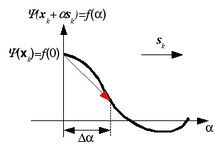
  (a) Failed to parse (SVG (MathML can be enabled via browser plugin): Invalid response ("Math extension cannot connect to Restbase.") from server "https://wikimedia.org/api/rest_v1/":): {\displaystyle f(\Delta\alpha)<f(0)} and Failed to parse (SVG (MathML can be enabled via browser plugin): Invalid response ("Math extension cannot connect to Restbase.") from server "https://wikimedia.org/api/rest_v1/":): {\displaystyle f'(\Delta\alpha)f'(0)>0}

• 

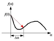
  (b) Failed to parse (SVG (MathML can be enabled via browser plugin): Invalid response ("Math extension cannot connect to Restbase.") from server "https://wikimedia.org/api/rest_v1/":): {\displaystyle f(\Delta\alpha)<f(0)} and Failed to parse (SVG (MathML can be enabled via browser plugin): Invalid response ("Math extension cannot connect to Restbase.") from server "https://wikimedia.org/api/rest_v1/":): {\displaystyle f'(\Delta\alpha)f'(0)<0}

• 

  (c) Failed to parse (SVG (MathML can be enabled via browser plugin): Invalid response ("Math extension cannot connect to Restbase.") from server "https://wikimedia.org/api/rest_v1/":): {\displaystyle f(\Delta\alpha)>f(0)}

In case (a), keep searching the optimal α in the same direction. you may increase the step size for fast search. In case (c), reduce the step size by half, and perform the next search. In case (b), interpolate f(α) with the quadratic spline and set α_k that minimizes the spline. Note that the slope of a function f(α), df/dα corresponds to the dot product of the gradient vector at α with the search direction, or

Failed to parse (SVG (MathML can be enabled via browser plugin): Invalid response ("Math extension cannot connect to Restbase.") from server "https://wikimedia.org/api/rest_v1/":): {\displaystyle \frac{df(\alpha)}{d\alpha} = \mathbf{s}_k^T\mathbf{g}(\mathbf{x}_k + \alpha\mathbf{s}_k)} .

In zxcgr, the maximum iteration number for the line search is set as MAXLIN = 5 in the relax_zxcgr.cpp file. If the line search cannot find an α that reduces the function f within 5 consecutive iterations, the following error message will be printed: "CGRelax: Line search aborted"

PR+

PR+ routine was added by Keonwook Kang in 2009 based on LAMMPS's min_cg.cpp file. The update parameter is β^PR+. For the line search method, the backtracking method is used. The backtracking method does not guarantee that a function f minimizes at the obtained α. This method allows any step size that can sufficiently decrease the function f. This decision can be justified if it is undesirable or impossible to exactly minimizes a function f or if we do not want to spend too much computation time to find an exact α.

Comparision of the CG methods in different implementation

In the first part of this section, I compare the computation results obtained from CG relxation between MD++ (ver.Mar202009) and LAMMPS (ver.Mar262009). The test system is a 3[100] x 3[010] x 3[001] Si diamond cubic structure stretched by 10% in all three directions with two missing atoms (of atom ID 0 and 99). The number of atoms in the test system is 8x3³ - 2 = 214. The potential fuction is MEAM Siz with the cut-off radius r_c=6(Å). The CG method is implemented by using the Polak-Ribiere method (PR+) and the backtracking method. The energy and the force tolerances are given as etol = 1e-6 (no unit) and ftol = 1e-8 (eV/Å), respectively. In the 1st column of table 2, the potential energies of the perfect structure from MD++ and LAMMPS are compared, and they are identical. In the 2nd column, the potential energies of the defect structure before relaxation are compared, and they are again same. In the 4th column, the energies of the relaxed structure are listed in different colors depending on the values of d_max (0.1, 0.01, and 0.001), which are related with the initial step length, and we can say that the both results are effectively identical. For this small test system, MD++ is faster than LAMMPS, because of less evaluation of the potential function. For a larger system, LAMMPS can perform better due to its ability of parallel run.

Table 2. Relaxation of 3[100]x3[010]x3[001] Si structure with a defect. Potential file : MEAM Siz w/ r_c = 6 (A). CG method = (PR+) + (backtracking). Conditions: etol = 1e-6 (no unit), ftol = 1e-8 (eV/Å). Compiler = intel compiler

	Eperf (eV)	Edefect (eV)	dmax (Å)	Erlx (eV)	Iter. No.	No. of Calls	CPU time
MD++ (PR+)	-1.00008000022397e+03	-9.00066105589930e+02	0.1	-9.04000029718829e+02	15	46	0.30002
			0.01	-9.04000167032814e+02	46	51	0.33202
			0.001	-9.03987772936424e+02	424	425	2.2201
LAMMPS (Serial Run)	-1.00008000022397e+03	-9.00066105589930e+02	0.1	-9.04000029718830e+02	15	60	0.75296
			0.01	-9.04000167032815e+02	46	96	1.2149
			0.001	-9.03987772936423e+02	424	848	10.281

The distinct difference of the CG method between MD++ and LAMMPS lies in the fact that MD++ runs the CG method in scaled coordinate (x^*) while LAMMPS does in real coordinate (x). Because of this scaling effect, d_max must be devided by the box length L for MD++, or d^*_max = d_max/L. By the same reason, the force tolerance in MD++ needs to be multiplied by the box length, or ftol^* = L·ftol.

Now, I compare zxcgr and PR+ in MD++. Since it is only the force tolerance that the "zxcgr" code considers to check the convergence, the energy tolerance will be set to be 0 in the comparison below. In table 3, the numbers are same upto 1e-8. Note that the energy obtained by the PR+ method becomes lower than the number (in table 2) from the same method with nonzero etol (=1e-6). This further relaxation can be understood, if we consider that in the case of nonzero energy tolerance a small step makes the energy change small enough to satisfy the energy tolerance and the system is prone to stop relaxing further even though it is able to do because of its nonzero gradient (or force).

Table 3. Relaxation of 3[100]x3[010]x3[001] Si structure with a defect. Potential file : MEAM Siz w/ r_c = 6 (A). Conditions: etol = 0 (no unit), ftol = 1e-4 (eV/Å).

	dmax (Å)	Erlx (eV)	Iter. No.	No. of Calls	CPU time
MD++ (zxcgr)		-9.04000245866814e+02	31	45	0.31602
MD++ (PR+)	0.1	-9.04000245866095e+02	35	124	0.70004
	0.01	-9.04000245869413e+02	63	117	0.70004
	0.001	-9.04000245869795e+02	460	483	2.6002

At this point, we may raise a question. Does the scaling effect ever affect the relaxation of a structure in a non-cubic cell? Let's say that we have a 6[100] x 3[010] x 3[001] Si diamond cubic structure stretched by 20% in x direction with two missing atoms (of atom ID 0 and 99). The relaxation results are listed in table 4 below.

Table 4. Relaxation of 6[100]x3[010]x3[001] Si structure with a defect. Potential file : MEAM Siz w/ r_c = 6 (A). Conditions: etol = 0 (no unit), ftol = 1e-4 (eV/Å). For the PR+ method, d_max = 0.1 (Å). No. of atoms = 430

	Eperf (eV)	Edefect (eV)	Erlx (eV)	Iter. No.	No. of Calls
MD++ (zxcgr)	-2.00016000044795e+03	-1.86579478735442e+03	-1.86764046397026e+03	129	175
MD++ (PR+)			-1.86764046392565e+03	168	686
LAMMPS	-2.00016000044795e+03	-1.86579478735442e+03	-1.86764046393067e+03	74	387

The relaxed energy values are same upto 1e-6.

Issues with a structure of multiple local minima

If a structure has multiple local minima that are closely located, can we get the same relaxed structure with different CG methods? A Si slab can easily have multiple metastable structures because of the surface reconstruction and for that reason it is a good test system for our purpose. The simulation systems are 5[100]x5[010]x2[001] Si slabs: one with a surface atom of ID 142 intentionally removed and the other with not. (See figure 3.) Both systems are relaxed with zxcgr and PR+ CG methods, and the results are summarized in table 5.

The Si slab with no atom removed was able to reach the same metastable structure regardless of CG methods. However, in the other slab the removed atom triggered the surface atoms' bonding or de-bonding differently depending on the CG method. Apparently, we observe two different surface reconstruction patterns obtained from the same initial structure.

Table 5 Relaxation of a 5[100]x5[010]x2[001] Si slab. Potential file : MEAM Siz w/ r_c = 6 (A). Conditions: etol = 0 (no unit), ftol = 1e-4 (eV/Å).

CG	System 1 (No atom removed)			System 2 (1 atom removed)
	Iter. No.	No. of Calls	Erlx (eV)	Iter. No.	No. of Calls	Erlx (eV)
zxcgr	13	29	-1.69159677459827e+03	189	328	-1.72478726205782e+03
PR+	44	183	-1.69159677459797e+03	571	1255	-1.72304961624534e+03

Figure 3

	Initial structure of System 1	Initial structure of System 2	Relaxed structure of System 2
			zxcgr	PR+
top view
side view

How do we interprete this behavior? If a given object function has multiple local minima that are very close, a slightly different search path can lead you different energy valleys. This idea can be confirmed by relaxing structures with another Si potential, Stillinger-Weber (SW), which is less bumpy than MEAM. The relaxation results are shown below in table 6 and figure 4. According to the results, both zxcgr and PR+ methods give the same relaxed structure of the system 2 in terms of energy and the surface pattern. Note that the relaxed structures do not show any appreciable surface reconstruction.

Table 6 Relaxation of a 5[100]x5[010]x2[001] Si slab with SW Potential. CG Conditions: etol = 0 (no unit), ftol = 1e-4 (eV/Å).

CG	System 1 (No atom removed)			System 2 (1 atom removed)
	Iter. No.	No. of Calls	Erlx (eV)	Iter. No.	No. of Calls	Erlx (eV)
zxcgr	6	10	-1.62049999855975e+03	7	11	-1.61586999856701e+03
PR+	7	37	-1.62049999855992e+03	7	37	-1.61586999856631e+03

Figure 4 Images of relaxed structures with SW potential

	Relaxed structure of System 2
	zxcgr	PR+
top view
side view

This comparison does not mean that SW potential performs better than MEAM or the other way around. We just want to point out that there is a feature of a potential function that may unintendedly affect the relaxation results, and we have to be very careful when taking them.