Manual 05 for MD++
MD++ Tour with Sample Scripts
Keonwook Kang and Wei Cai
[First written, [ Jan 19 ]], 2007
[Last Modified, [ Feb 25 ]], 2008
Contents |
Molecular Dynamics Simulation
In Manual 02, we learned how to create a perfect BCC, FCC or DC crystal by the MD++ command makecrystal, by which we assigned the initial position to each of the atoms. For nonzero finite temperature simulation or molecular dynamics (MD) simulation, we need to additionally give the initial velocities and set quite a few variables such as numerical integrator, time step, total steps, atomic mass as well as other parameters that controls the simulation output. In this manual, we aim to make you feel familiar with MD++ commands and variables related with MD simulations. MD simulations can be categorized as microcanonical (NVE), canonical (NVT), isoenthalpic-isobaric (NPH) and constant pressure/temperature (NPT) ensemble types according to which physical quantities are expected to be constant or controlled. For example, a system of microcanonical ensemble has the total energy (E), the system volume (V) and the number of atoms (N) to be conserved during MD simulation. Basically, you need to choose a proper ensemble set for your own purpose of simulation.
Microcanonical(NVE) Ensemble
It would be a good start explaining MD simulation of NVE ensemble to understand what you do with MD simulations. Imagine a system of N-particle gas inside of a rigid container which is well insulated that the system is isolated from the environment. There is no heat and mass transfer through the container wall. Then you expect that the number of particles, the container volume and the total energy will not change. In MD simulations of NVE ensemble, you do not see a visible wall but you may think of a closed system with fictitious walls.
Now I give the example script mo_NVE.tcl below, written in Tcl version. You can run the script by typing
$ bin/fs_gpp scripts/mo_NVE.tcl
and it first creates a perfect BCC crystal of molybdenum (Mo) with a supercell of 5[1 0 0] X 5[0 1 0] X 5[0 0 1] and then runs MD simulations using the Finnis-Sinclair (FS) potential.
# -*-shell-script -*-
# run NVE MD simulation of perfect crystal of Mo.
#
#*******************************************
# Definition of procedures
#*******************************************
proc initmd { } { MD++ {
#setnolog
setoverwrite
dirname = runs/mo-example
zipfiles = 1   # zip output files
#
#--------------------------------------------
# Create Perfect Crystal
element0 = Mo
crystalstructure = body-centered-cubic
latticeconst = 3.1472           # in Angstrom for Mo
latticesize = [ 1 0 0 5
                0 1 0 5
                0 0 1 5]
}}
#------------------------------------------------------------
proc readMoPot { } { MD++ {
# Read the potential file
potfile = ~/Codes/MD++/potentials/mo_pot readpot
}}
#-------------------------------------------------------------
proc openwindow { } { MD++ {
# Plot Configuration
atomradius = 1.0 bondradius = 0.3 bondlength = 2.725
atomcolor = orange highlightcolor = purple
bondcolor = red backgroundcolor = gray70
plotfreq = 10 rotateangles = [ 0 0 0 1.25 ]
openwin alloccolors rotate saverot eval plot
}}
#--------------------------------------------
proc setup_md { } { MD++ {
#MD settings
ensemble_type = "NVE" integrator_type = "VVerlet"
T_OBJ = 300        # (in Kelvin) Desired Temperature
atommass = 95.94   # (in g/mol)
timestep = 0.001   # (in ps)
totalsteps = 2000
# save property every 10 steps
saveprop = 1 savepropfreq = 10
savecn = 0   savecnfreq = 100
writeall = 1 DOUBLE_T = 1
randseed = 12345 srand48 #randomize random number generator

#*******************************************
# Main program starts here
#*******************************************
initmd
readMoPot
MD++ makecrystal finalcnfile = perf.cn writecn
openwindow
#---------------------------------------------
# run MD
setup_md
MD++ initvelocity finalcnfile = init.cn writecn
#format of thermodynamic property file
MD++ {output_fmt = "curstep EPOT KATOM Tinst"}
MD++ outpropfile = thermo.out openpropfile
MD++ run closepropfile
MD++ finalcnfile = 300K-5X5X5.cn writecn eval
MD++ sleep quit
}}
In the fuction setup_md { } in the above script, important MD++ parameters for MD simulations are assigned. First, you choose which ensemble you impose by specifying ensemble_type to be NVE, NVT, NPH or NPT. You also decide the integrator between Gear 6-th order predictor-corrector and velocity Verlet by saying integrator_type = "Gear6" or integrator_type = "VVerlet". The predictor-corrector integrator has higher order of accuracy but the Verlet integrator is symplectic and is believed to be resilient to the larger time step.
atommass is the atomic mass in g/mol, timestep is Δt used in the integrator in the unit of picosecond, totalsteps is the total number of iterations in time integration. As long as it is guaranteed that the total energy of the system is conserved, the timestep (timestep) is usually taken as big as possible. The total time step (totalsteps) is typically chosen long enough for the system to reach its dynamical steady state.
The initial velocity is first assigned as random numbers but then scaled to correspond to an instantaneous temperature of T_OBJ.<ref>T_OBJ is the target temperature in NVT ensemble. However, it is used here just to generate atoms' initial velocities and that does not necessarily mean the temperature will be maintained at the specified value during the simulation because there is no temperature we control in NVE ensemble.</ref> The MD++ command initvelocity initializes the velocity to each atom randomly according to the value of T_OBJ. For random number generation, srand48 is executed with an integer random seed randseed. Running the simulation again with the same randseed will give you the same result (which is good for debugging). Running the simulation again with a different randseed will give you a different initial velocity condition (which is good for collecting statistics). You may also use the MD++ command srand48bytime, which will use the current time as the random seed (in this way, your simulation will always have a different initial velocity condition whenever you run it again).
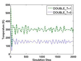
If the parameter DOUBLE_T is set to be 1, the initial temperature becomes twice. You can see the effect of DOUBLE_T = 1 in Fig.1. When you see the temperature plot in Fig.1, you will realize that the temperature at equilibrated state seems to be half of the initial temperature. The reason why the temperature reduces by half is followed. Since the initial atomic configuration at 0 K is the local-energy-minimum structure, part of the kinetic energy initially given is always converted to the potential energy during MD simulation and this portion amounts to be half of the kinetic energy.
 . .
|
for 3D case due to the equipartition theorem.
- Fig.1 The effect of DOUBLE_T
The MD++ command run starts MD simulation with all these parameters. There are more parameters related with MD simulation. saveprop and savepropfreq will determine whether or not the thermodynamic properties will be written in file and how often they will be. If saveprop = 1 and savepropfreq = 10, the thermodynamic properties such as potential energy, kinetic energy and temperature will be dumped out at every 10 step only if the MD++ command openpropfile is executed.
The content of a property file is defined by output_fmt. Accordig to the example script, each line of the property file contains current step (curstep), potential energy (EPOT), kinetic energy (KATOM), and temperature (Tinst). If we do not specify output_fmt, the default array of thermodynamic data output is current step (curstep), kinetic energy (KATOM), potential energy (EPOT), pressure (PRESSURE), -σxy (TSTRESS_xy), -σyz (TSTRESS_yz), -σzx (TSTRESS_zx), HELM, the extended energy(HELMP), thermodynamic friction coefficient (zeta), dEdlambda and the system volume (OMEGA). Units are given as eV for energy and eV/A˚^3 for stress. The sign of the stress TSTRESS is the opposite of the conventional definition in elasticity or continuum theory, because MD++ is implemented following Parrinello and Rahman's definition of stress.<ref>M. Parrinello and A. Rahman, "Polymorphic transitions in single crystals: A new molecular dynamics method", J. Appl. Phys 52 7182-7190 1981</ref>
The thermodynamic properties can be loaded and plotted by the external program such as Octave and Matlab.<ref>A simple way to plot the total energy using gnuplot (a free software on Unix/Linux) is to run the command.
plot "prop.out" u ($1):($2+$3) with line
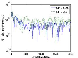
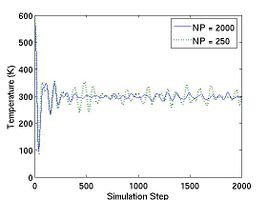
</ref> In Fig.2, total energy per atom and temperature are plotted for the systems of two different size. The bigger system (10[100] X 10[010] X 10[001]) has eight times more atoms than the other (5[100] X 5[010] X 5[001]). Obviously, you see that the thermodynamic data in the bigger system show less fluctuation.
- Fig.2 Energy and Temperature fluctuation of NVE ensemble
savecn and savecnfreq are used to determine how often the intermediate configuration will be saved as .cn file with the MD++ command openintercnfile just like saveprop and savepropfreq. You can specify names of the property file and the intermediate configuration files using MD++ parameter outpropfile and intercnfile, respectively. If we do not specify them, the default file name would be prop.out and inter.cn. The expression zipfiles = 1 in the 11th line will compress files such as .out and .cn. For example, the configuration file init.cn and the thermodynamic data file thermo.out will be zipped as init.cn.gz and thermo.out.gz, respectively.
Calling writecn saves a configuration (.cn) file, which contains the following informations; The first line specifies the total number of atoms (NP). After that there are NP lines of data and each line has three columns in default, which correspond to the scaled coordinate (sx, sy, sz) of one atom. And then there are three lines of data that specifies a 3 X 3 box matrix  . The real coordinates of an atom (x, y, z ) and the scaled coordinates are related by the following
 . .
|
If writeall = 1, additional informations are added to NP lines of data such that each line has sacaled velocities (_VSR[i].x, _VSR[i].y and _VSR[i].z), individual potential energy (_EPOT_IND[i]), whether-or-not fixed (fixed[i]), topology (_TOPOL[i]), atom species (species[i]), atom groups (group[i]) and images (image[i]) after the scaled coordinates(_SR[i].x, _SR[i].y and _SR[i].z for i=1 to NP) . You can check this difference by comparing two configuration files, perf.cn and init.cn. Because perf.cn is written before setting writeall = 1, it has only number of atoms, scaled coordinates of each atom and the box matrix  while init.cn has all the informations. Alternatively, writevelocity = 1 can be used, which stores only the scaled coordinates and the scale velocities.
Commands and variables related with visualization in openwindow will be covered in a separate manual in detail.
After the simulation (run) has finished, the sleep command allows the graphics window to stay alive for a while so that we can look at the final atomic structure. You can press ctrl-c in the terminal to exit. You can also comment out the sleep command so that MD++ quits right after finishing run.
Canonical(NVT) Ensemble
The following example script mo_NVT.tcl reads the structure file of BCC Mo and runs NVT MD simulation during which temperature is maintained at 300 K using Nose-Hoover thermostat<ref> S. Nose, “A Molecular Dynamics Method for Simulations in the Canonical Ensemble”, Molecular Physics, 52 255 (1984)</ref>. Run the script by typing
$ bin/fs_gpp scripts/mo_NVT.tcl
# -*-shell-script -*-
# run NVT MD simulation of perfect crystal of Mo.
#
#*******************************************
# Definition of procedures
#*******************************************
proc initmd { } {
         ...
}
#------------------------------------------------------------
proc readMoPot { } {
         ...
}
#-------------------------------------------------------------
proc openwindow { } {
         ...
}
#--------------------------------------------
proc setup_md { } { MD++ {
#MD settings
ensemble_type = "NVT" integrator_type = "VVerlet"
implementation_type = 0 vt2 = 1e28
T_OBJ = 300       # (in Kelvin) Desired Temperature
atommass = 95.94  # (g/mol)
timestep = 0.001 # (ps)
totalsteps = 2000
saveprop = 1 savepropfreq = 10
savecn = 0 savecnfreq = 100
writeall = 1
}}
#*******************************************
# Main program starts here
#*******************************************
initmd
readMoPot
MD++ {
  incnfile = 300K-5X5X5.cn
  atommass = 95.94 timestep = 0.001
  readcn eval
}
openwindow
#---------------------------------------------
# run MD
setup_md
MD++ {output_fmt = "curstep EPOT KATOM Tinst HELMP"}
MD++ outpropfile = thermo-NVT.out openpropfile
MD++ run eval
#reverse velocity (to test reversibility)
MD++ input = -1 multiplyvelocity
#MD simulation (reverse)
MD++ run eval
MD++ finalcnfile = 300K-5X5X5-NVT.cn writecn
MD++ sleep quit
Instead of creating BCC Mo crystal, this script reads the configuration file 300K_5X5X5.cn, which was generated by the previous script mo_NVE.tcl, using the MD++ command readcn. Note that when MD++ reads the configuration file, the timestep should be idnetical with that of the previous run because the scaled velocity is stored as dimensionless unit after being multiplied with the timestep. It is safe that you specify timestep and atommass when reading .cn file as shown in the script.
Setting ensemble_type = "NVT" activates Nose-Hoover thermostat, which basically adds one more degree of freedom (ζ) to the system such that the temperature is controlled by feedback routine by allowing heat transfer to the heat reservoir,
 . .
|
when the degree of freedom is 3N. In MD++, Nose-Hoover thermostat are implemented in three different way, each of which uses different integrator defined through implementation_type. If it is zero, the implicit integrator will be chosen. If it is one, the explicit integrator based on Sto¨rmer-Verlet method will work. If it is two, another explicit integrator based on Liouville formulation will be activated.
Thermal coefficient vt2 is related with thermal mass Q of Nose´-Hoover thermostat as
 . .
|
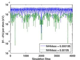
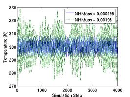
where N is number of atoms and k_B is the Boltzmann constant (8.617343e-5 eV/K). For convenience, we also defined thermal mass NHMass, which is exactly Nose'-Hoover thermal mass Q. When N = 250 and T = 300 K (or k_B T ~ 0.026 eV), vt2 = 1e28 corresponds to NHMass = 1.95e-03. The bigger vt2 is (or the smaller NHMass is), the faster the response of the system is to control the temperature. The effect of vt2 on Helmholtz free energy and temperature fluctuation is shown in Fig. 3.
- Fig.3 The Effect of Nose-Hoover Mass in NVT MD
HELMP in the output_fmt is Helmholtz free energy which is the conserved quantity in NVT MD.
multiplyvelocity multiplies the number specified by the preceding input to all velocity components of all atoms. With input=-1, the MD++ command multiplyvelocity reverses the velocity direction of all the atoms and they are expected to be at the initial position after the reverse run. This is done to test the reversibility of the symplectic integrator. Comparing two configuration files 300K-5X5X5.cn and 300K-5X5X5-NVT.cn reveals that the numbers become different after 10^(-14) digit. If we consider the total step is 4000, the difference at each step would be O(10^(-17)), which corresponds to the machine precision. We can say the symplectic integrator is indeed reversible.
Isoenthalpic-isobaric (NPH) Ensemble
