ShElastic Manuals

ShElastic is the python code for the paper

Wang, Y., Zhang, X., & Cai, W. (2019). Spherical Harmonics Method for Computing the Image Stress Due to A Spherical Void. Journal of the Mechanics and Physics of Solids.

The code is tested under Ubuntu 16.04 LTS. with package python 3.6, numpy 1.15, scipy 1.0, matplotlib 3.0, jupyter, and SHTOOLS 4.3. Please see Install_SHTOOLS for more details on installing required packages

Obtain the ShElastic package

Please download the package using git:

git clone https://gitlab.com/micronano/ShElastic.git

or directly from https://gitlab.com/micronano/ShElastic

Suggested Installation of SHTOOLS (pip)

If you have python3 and pip installed on your machine, you can simply install everything by:

python3 -m pip install --user numpy scipy matplotlib ipython jupyter pandas sympy nose pyshtools

Generate coefficients

The coefficients up to l_{max} = 60 is pre-computed and included in the repository. If you want to use higher mode spherical harmonic basis, please continue reading.

Please change the first few lines in `ShElastic/scripts/generate_modes.py`:

lKfull = 10
lJfull = lKfull + 3
savepath = '../module/lmax%dmodes'%lKfull
...

Then we can generate the mode files by calling:

cd ShElastic/scripts
python3 generate_modes.py

The mode files will be saved in the savepath folder.

Reproduce results from the paper

The results showing in the paper can be reproduced by running the jupyter notebooks in `ShElastic/notebook` folder.

Numerical Case 1: `Case01-Uniform_Tensile_Hole.ipynb` Numerical Case 2: `Case02-Void_Dislocation_Interaction.ipynb` Numerical Case 3: `Case03-Prismatic_Dislocation_Loop.ipynb`

Launch the jupyter notebook by:

cd ShElastic
jupyter notebook

The result files will be saved in `ShElastic/figures`. The figures in the paper can be reproduced by running plotdata.m in matlab.

• Fig.1 generated figures for the paper
• 

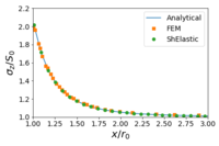
  (a) Case 1

• 

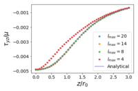
  (b) Case 2

• 

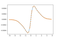
  (c) Case 3