ShElastic Manuals: Difference between revisions
(Created page with "[https://gitlab.com/micronano/ShElastic ShElastic] is the python code for the paper Wang, Y., Zhang, X., & Cai, W. (2019). Spherical Harmonics Method for Computing the Image ...") |
No edit summary |
||
| Line 13: | Line 13: | ||
or directly from https://gitlab.com/micronano/ShElastic |
or directly from https://gitlab.com/micronano/ShElastic |
||
== |
== Suggested Installation of SHTOOLS (pip) == |
||
If you have python3 and pip installed on your machine, you can simply install everything by: |
|||
On mc2 cluster, since we can only install packages for user only, we are not allowed to use sudo command to install the required packages. We need to compile the packages by our own. |
|||
python3 -m pip install --user numpy scipy matplotlib ipython jupyter pandas sympy nose pyshtools |
|||
For compiling shtools, the required packages are fftw3, lapack, and blas. Libraries for lapack and blas are available on mc2, we can use them directly for compiling shtools. For installing fftw3, please refer to [http://micro.stanford.edu/wiki/Install_FFTW3 Install_FFTW3] for more details. |
|||
== Generate coefficients == |
|||
After you followed the steps in FFTW3 installation (Serial only), you should have all the fftw3 libraries available: |
|||
The coefficients up to $l_{max} = 60$ is pre-computed and included in the repository. If you want to use higher mode spherical harmonic basis, please continue reading. |
|||
~/usr/include/fftw3.h |
|||
~/usr/include/fftw3.f |
|||
~/usr/lib/libfftw3.a |
|||
~/usr/lib/libfftw3.la |
|||
~/usr/lib/libfftw3.so |
|||
Please change the first few lines in `ShElastic/scripts/generate_modes.py`: |
|||
And also, run the command: |
|||
lKfull = 10 |
|||
ls /usr/lib64 |
|||
lJfull = lKfull + 3 |
|||
savepath = '../module/lmax%dmodes'%lKfull |
|||
The libraries for lapack and blas should be available here: |
|||
/usr/lib64/liblapack.a |
|||
/usr/lib64/liblapack.so |
|||
/usr/lib64/liblapack.so.3 |
|||
... |
... |
||
/usr/lib64/libblas.a |
|||
/usr/lib64/libblas.so |
|||
/usr/lib64/libblas.so.3 |
|||
... |
|||
Before we proceed, we need to make sure to have python installed. |
|||
=== Install python + scipy + SHTOOLS on local directory === |
|||
We create a local folder .localpython for installing python: |
|||
mkdir ~/.localpython |
|||
download python source code: |
|||
mkdir ~/soft |
|||
cd ~/soft |
|||
wget http://www.python.org/ftp/python/X.X.X/Python-X.X.X.tgz |
|||
tar -xvf Python-X.X.X.tgz |
|||
cd Python-X.X.X |
|||
compile python from source and install to local directory: |
|||
make clean |
|||
./configure --enable-shared --prefix=${HOME}/.localpython |
|||
make |
|||
make install |
|||
Add the following lines to ~/.bashrc: |
|||
export PATH=${HOME}/.localpython/bin:$PATH |
|||
export PYTHONPATH=${HOME}/.localpython/bin |
|||
export LIBRARY_PATH=$LIBRARY_PATH:${HOME}/.localpython/lib |
|||
export LD_LIBRARY_PATH=$LD_LIBRARY_PATH:${HOME}/.localpython/lib |
|||
if python version < 2.7.9, install pip by: |
|||
wget https://bootstrap.pypa.io/get-pip.py |
|||
python get-pip.py |
|||
export PATH=${HOME}/.local/bin:$PATH |
|||
Install SciPy Stack using pip on user's directory: |
|||
pip(pip3) install --user numpy scipy matplotlib ipython jupyter pandas sympy nose |
|||
Install pyshtools using pip: |
|||
First, we put the pre-compiled FFTW3 libraries into LIBRARY_PATH: |
|||
export LIBRARY_PATH=$LIBRARY_PATH:${HOME}/usr/lib |
|||
export LD_LIBRARY_PATH=$LD_LIBRARY_PATH:${HOME}/usr/lib |
|||
Then we can install pyshtools through pip on user's directory: |
|||
pip(pip3) install --user pyshtools |
|||
=== Compile SHTOOLS === |
|||
load the python module (we use python 2 as an example): |
|||
module load python/2.7.8 (Whichever is available) |
|||
Also make sure you have numpy available: |
|||
pip list |
|||
Then you are ready to install shtools on your mc2 account. |
|||
First, download the shtools source package from [https://github.com/SHTOOLS/SHTOOLS/releases Releases] |
|||
cd ~/soft |
|||
wget https://github.com/SHTOOLS/SHTOOLS/archive/v3.4.tar.gz |
|||
tar -zxvf v3.4.tar.gz |
|||
cd SHTOOLS-3.4 |
|||
Then, indicate the libraries and compile the source code: |
|||
export LD_LIBRARY_PATH=$LD_LIBRARY_PATH:"$HOME/usr/lib" |
|||
make python2 LAPACK="-L/usr/lib64 -llapack" BLAS="-L/usr/lib64 -lblas" FFTW="-L$HOME/usr/lib -lfftw3" |
|||
The output should be something look like [https://shtools.oca.eu/shtools/www/makeout.html this]. Then your package is ready for use. If you are compiling with python 3, just change "python2" to "python3" in the command above. |
|||
To load the SHTOOLS module in python, use the following lines: |
|||
import sys |
|||
sys.path.append('$HOME/soft/SHTOOLS-3.4') |
|||
import pyshtools as shtools |
|||
where the "$HOME" has to be substituted by your own home folder path. |
|||
== Examples for using SHTOOLS in python == |
|||
We consider a simple example where we do the spherical expansion of function <math>x^2</math> on the surface of a unit sphere. |
|||
First we import the necessary packages: |
|||
from __future__ import print_function # only necessary if using Python 2.x |
|||
import numpy as np |
|||
import sys |
|||
sys.path.append('/home/yfwang09/soft/SHTOOLS-3.4') |
|||
import pyshtools as psh |
|||
Then we generate the mesh grids for the spherical coordinates (Nx2N grids for latitude and longitude variables <math>\phi, \theta</math>; or <math>\pi/N</math> latitudinal and <math>2\pi/2N</math> longitudinal, both start from 0): |
|||
Ngrid = 100 |
|||
phi = np.linspace(0, np.pi, Ngrid) |
|||
theta = np.linspace(0, 2*np.pi, 2*Ngrid) |
|||
THETA, PHI = np.meshgrid(theta, phi) # make the grid size as Nx2N |
|||
where the grid PHI and THETA both have N rows and 2N columns. Then we translate the Cartesian coordinates into the spherical meshgrids, and generate the target function into spherical coordinates: |
|||
Z = np.cos(PHI); |
|||
X = np.sin(PHI)*np.cos(THETA); |
|||
Y = np.sin(PHI)*np.sin(THETA); |
|||
X2 = X**2 |
|||
Finally we expand the target function into spherical harmonic series: |
|||
cilm = np.empty([2,Ngrid/2,Ngrid/2]) |
|||
filename = 'xsquare' |
|||
cilm = psh.expand.SHExpandDH(X2, sampling=2) |
|||
np.savetxt(filename+'_clm.txt', cilm[0,:,:], header='Row: l, Column: m') |
|||
np.savetxt(filename+'_slm.txt', cilm[1,:,:], header='Row: l, Column: m') |
|||
Then we can generate the mode files by calling: |
|||
where cilm represent the coefficients of different spherical harmonic modes. cilm[0, l, m] and cilm[1, l, m] are the cosine and sine modes of spherical harmonics. The parameter sampling=2 means that we are using the grid Nx2N instead of NxN. |
|||
cd ShElastic/scripts |
|||
See the page [https://shtools.oca.eu/shtools/www/man/python/pyshexpanddh.html SHExpandDH] for the detailed description of the expanding function and the page [https://shtools.oca.eu/shtools/www/conventions.html Real Spherical Harmonics] for mathematical definition. |
|||
python3 generate_modes.py |
|||
The mode files will be saved in the savepath folder. |
|||
== Visualize spherical harmonic modes using scipy == |
|||
== Reproduce results from the paper == |
|||
We first import the necessary packages: |
|||
The results showing in the paper can be reproduced by running the jupyter notebooks in `ShElastic/notebook` folder. |
|||
import numpy as np |
|||
from scipy.special import sph_harm |
|||
import matplotlib.pyplot as plt |
|||
from matplotlib import cm, colors |
|||
from mpl_toolkits.mplot3d import Axes3D |
|||
Numerical Case 1: `Case01-Uniform_Tensile_Hole.ipynb` |
|||
For a certain pair of parameters (m, l), we can plot the corresponding spherical harmonic mode Y(l, m) on the surface of a unit sphere using scipy and matplotlib packages. Here we use the meshgrid THETA, PHI, X, Y, and Z we generated in the previous section: |
|||
Numerical Case 2: `Case02-Void_Dislocation_Interaction.ipynb` |
|||
Numerical Case 3: `Case03-Prismatic_Dislocation_Loop.ipynb` |
|||
Launch the jupyter notebook by: |
|||
fvalues = sph_harm(m, l, THETA, PHI).real # Get the values of spherical harmonic functions |
|||
fmax, fmin = fvalues.max(), fvalues.min() |
|||
fcolors = (fvalues - fmin)/(fmax - fmin) # normalize the values into range [0, 1] |
|||
cd ShElastic |
|||
Then we plot Y(l, m) on a sphere: |
|||
jupyter notebook |
|||
The result files will be saved in `ShElastic/figures`. The figures in the paper can be reproduced by running plotdata.m in matlab. |
|||
fig = plt.figure(figsize=plt.figaspect(1.)) # make the axis with equal aspects |
|||
ax = fig.add_subplot(111, projection='3d') # add an subplot object with 3D plot |
|||
ax.plot_surface(x, y, z, rstride=1, cstride=1, facecolors=cm.Blues(fcolors)) |
|||
plt.show() |
|||
For example, the figures for (l, m) = (2, 0), (3, 2), and (1, 1) are shown as below: |
|||
<gallery caption="Fig.1 Visualization of Spherical Harmonics" widths="200px" heights="200px" perrow="3"> |
<gallery caption="Fig.1 Visualization of Spherical Harmonics" widths="200px" heights="200px" perrow="3"> |
||
Image:sph_harm_Y20.png|(a) <math> Y_{20}(\theta,\phi) </math> |
Image:sph_harm_Y20.png|(a) <math> Y_{20}(\theta,\phi) </math> |
||
Revision as of 23:02, 19 February 2019
ShElastic is the python code for the paper
Wang, Y., Zhang, X., & Cai, W. (2019). Spherical Harmonics Method for Computing the Image Stress Due to A Spherical Void. Journal of the Mechanics and Physics of Solids.
The code is tested under Ubuntu 16.04 LTS. with package python 3.6, numpy 1.15, scipy 1.0, matplotlib 3.0, jupyter, and SHTOOLS 4.3. Please see Install_SHTOOLS for more details on installing required packages
Obtain the ShElastic package
Please download the package using git:
git clone https://gitlab.com/micronano/ShElastic.git
or directly from https://gitlab.com/micronano/ShElastic
Suggested Installation of SHTOOLS (pip)
If you have python3 and pip installed on your machine, you can simply install everything by:
python3 -m pip install --user numpy scipy matplotlib ipython jupyter pandas sympy nose pyshtools
Generate coefficients
The coefficients up to $l_{max} = 60$ is pre-computed and included in the repository. If you want to use higher mode spherical harmonic basis, please continue reading.
Please change the first few lines in `ShElastic/scripts/generate_modes.py`:
lKfull = 10
lJfull = lKfull + 3
savepath = '../module/lmax%dmodes'%lKfull
...
Then we can generate the mode files by calling:
cd ShElastic/scripts
python3 generate_modes.py
The mode files will be saved in the savepath folder.
Reproduce results from the paper
The results showing in the paper can be reproduced by running the jupyter notebooks in `ShElastic/notebook` folder.
Numerical Case 1: `Case01-Uniform_Tensile_Hole.ipynb` Numerical Case 2: `Case02-Void_Dislocation_Interaction.ipynb` Numerical Case 3: `Case03-Prismatic_Dislocation_Loop.ipynb`
Launch the jupyter notebook by:
cd ShElastic
jupyter notebook
The result files will be saved in `ShElastic/figures`. The figures in the paper can be reproduced by running plotdata.m in matlab.
- Fig.1 Visualization of Spherical Harmonics
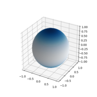
(a)
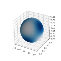
(b)
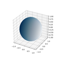
(c)


