M03 Equilibrium Lattice Constant and Bulk Modulus: Difference between revisions
(table caption and cetering) |
|||
| Line 125: | Line 125: | ||
number of atoms in the 3X3X3 cell is given in the following table. |
number of atoms in the 3X3X3 cell is given in the following table. |
||
{|class="wikitable" border="1" align="center" |
{|class="wikitable" border="1" align="center" |
||
| |
|+ Table 1. Number of atoms in different crystal structures |
||
| Crystal Structure || No. of atoms in the unit cell || Total No. of atoms |
|||
|- |
|- |
||
| |
|align="center"| SC ||align="center"| 1 ||align="center"| 27 |
||
|- |
|- |
||
| |
|align="center"| BCC ||align="center"| 2 ||align="center"| 54 |
||
|- |
|- |
||
| |
|align="center"| FCC ||align="center"| 4 ||align="center"| 108 |
||
|- |
|- |
||
| |
|align="center"| DC ||align="center"| 8 ||align="center"| 216 |
||
|} |
|} |
||
Revision as of 00:30, 27 November 2007
Manual 03 for MD++
Computing Equilibrium Lattice Constant
Keonwook Kang and Wei Cai
Reading a Log File
In the example scripts of Manual 02, the command setnolog was activated and the simulation results were printed out to the standard output, which is usually your terminal screen. If you want to keep the record of this information, you comment out the setnolog command by adding # before it. This will create a log file A.log in the directory specified by dirname. For example, if you run mo.script in Manual 02 with setnolog commented out, then you will find a A.log file in the runs/mo-example directory. To read this file, type
$ more runs/mo-example/A.log
In the log file, the line starting with ASSIGN shows that a variable is assigned to the values as specified in the script file. The line with EXEC shows the execution of certain command. After the eval command is executed, properties such as number of atoms (NP), potential energy (EPOT), kinetic energy (KATOM), pressure (PRESSURE) and stress (Stress) are also printed. Sometimes, the log file may be zipped as A.log.gz, in which case you can use
$ gzip -cd runs/mo-example/A.log.gz | more
to see the content. To search for a specific property (e.g. EPOT) in the log file, you may use
$ grep EPOT runs/mo-example/A.log
or
$ gzip -cd runs/mo-example/A.log.gz | grep EPOT
depending on whether the log file is zipped or not. In case you want to “grep” several lines before and after your keyword (e.g. Stress), you can use
$ grep -3 Stress runs/mo-example/A.log
This will show three lines above and below any line containing the keyword “Stress”.
Equilibrium Lattice Constant and Cohesive Energy
Under ambient condition silicon takes the diamond-cubic (DC) structure. But in a computer simulation, we can create Si crystals with different hypothet- ical structures, such as face-centered-cubic (FCC), body-centered-cubic (BCC), or simple-cubic (SC). A good potential model should be able to tell us that the DC structure is the one with the lowest energy, hence it is the most favorable structure for silicon. In this section, we will perform such calculations using MD++.
Let us define the lattice energy and the number density as


| . |
| . |


where is the potential energy of the crystal, is total number of atoms in the simulation cell (corresponding to variable NP in MD++) and is the volume of the simulation cell. Run MD++ with following command line to use the Stillinger-Weber (SW) potential model[1][2].


$ bin/sw gpp scripts/ME346/si_polytype.script
Here is the content of the si_polytype.script.
# -*-shell-script-*-
#setnolog
setoverwrite
dirname = runs/si_polytype
#------------------------------------------------------------
#Create Perfect Lattice Configuration
#
crystalstructure = diamond-cubic
latticeconst = 5.4309529817532409 #(A) for Si
latticesize = [ 1 0 0 3
                0 1 0 3
                0 0 1 3]
makecrystal eval
latticeconst = 4.850 makecrystal eval
latticeconst = 4.950 makecrystal eval
latticeconst = 5.050 makecrystal eval
                :
(many lines omitted here for brevity)
                :
latticeconst = 5.900 makecrystal eval
latticeconst = 6.000 makecrystal eval
latticeconst = 6.100 makecrystal eval
crystalstructure = face-centered-cubic
latticeconst = 4.105 makecrystal eval
latticeconst = 4.110 makecrystal eval
                :
                :
latticeconst = 4.205 makecrystal eval
latticeconst = 4.215 makecrystal eval
crystalstructure = body-centered-cubic
latticeconst = 3.210 makecrystal eval
latticeconst = 3.220 makecrystal eval
                :
                :
latticeconst = 3.320 makecrystal eval
latticeconst = 3.340 makecrystal eval
crystalstructure = simple-cubic
latticeconst = 2.550 makecrystal eval
latticeconst = 2.600 makecrystal eval
                :
                :
latticeconst = 2.640 makecrystal eval
latticeconst = 2.650 makecrystal eval
quit
From the log file, you can find number of atoms NP for the 3 X 3 X 3 DC cell to be 216. This number can also be obtained by calculating , since there are eight atoms in the DC unit cell. For other crystal structures, the number of atoms in the 3X3X3 cell is given in the following table.

| Crystal Structure | No. of atoms in the unit cell | Total No. of atoms |
| SC | 1 | 27 |
| BCC | 2 | 54 |
| FCC | 4 | 108 |
| DC | 8 | 216 |
The potential energy at each different lattice constant can also be read from the log file by typing
$ grep EPOT runs/si_polytype/A.log
The volume of a simulation cell can be obtained from the determinant of the matrix .[3] When is a diagonal matrix (the same is true for an upper triangular matrix),

| . |

the volume is the product of the entries in the main diagonal of \mathbf{H}. The unit of length in MD++ is Å and the unit of volume is Å3 . From these, we can calculate the lattice energy (in eV) of silicon as a function of the number density (in 1/Å3), for different crystal structures, as shown in Fig.1. The structure with the lowest energy is DC. The equilibrium lattice constant corresponds to the number density that gives the minimum of the curve. The minimum of is also called the cohesive energy . For DC silicon, 5.431 Å and = −4.63 eV.


- Fig.1 Visualization of FCC structure
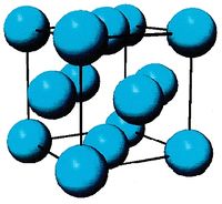
(a) Conventional image of FCC unit cell
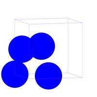
(b) FCC unit cell in MD++. One corner atom and three face-centered atoms per cell
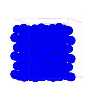
(c) FCC of 3X3X3 cells


Bulk Modulus
The curvature of the curve near the minimum also tells us the bulk modulus of the crystal. The bulk modulus is defined as[4]

| . |

where is the equilibrium atomic volume (corresponding to the energy minimum). To compute the second derivative, plot as a function of and fit the curve in the neighborhood of the minimum by a quadratic function, i.e. , as shown in Fig.1(b). This can be done by the Matlab command polyfit and the result is c2 = 0.0169 (in unit of eV/Å6 ). Then, with 20.025 (Å6), the bulk modulus becomes


| . |

This result matches with an earlier report in the literature[2]. In the elasticity theory[5], the bulk modulus is related to the other elastic constants through
| for isotropic material | |
| for cubic material |


where and are Lamé's constants and and are cubic elastic constants. From this relation, the bulk modulus would be 98.4 GPa if we calculate it from the experimental value of 165.7(GPa) and 63.9(GPa) for silicon. The discrepancy between the simulation and experimental results in the bulk modulus is partly because the simulation results corresponds to the ideal case of T = 0 K, while the experimental result is obtained at room temperature T = 300 K. The elastic constants generally decreases with increasing temperature. The discrepancy may also come from the fact that the potential model has empirical nature. Different parameterization of the potential model generally leads to different predictions of the elastic constants.


Notes
- ↑ F. H. Stillinger and T. A. Weber, Phys. Rev. B 31, 5262 (1985).
- ↑ 2.0 2.1 H. Balamane, T. Halicioglu, and W. A. Tiler, Phys. Rev. B 46, 2250 (1992)
- ↑ The matrix defines size and shape of the simulation cell. where 's are three periodicity vectors. In MD++, the matrix becomes a diagonal matrix when the supercell is a rectangular box (after reorienting the coordinate system).
- ↑ This is because Failed to parse (syntax error): {\displaystyle B = − V P / V } and Failed to parse (syntax error): {\displaystyle P = − \Phi / V} .
- ↑ J. P. Hirth and J. Lothe, Theory of Dislocations, (Wiley, New York, 1982)
![{\displaystyle \mathbf {H} =[\mathbf {c} _{1}\;\mathbf {c} _{2}\;\mathbf {c} _{3}]}](https://wikimedia.org/api/rest_v1/media/math/render/svg/0c0c26f5089c9bf30d4a63f25537c3b38b022f05)
