ShElastic Manuals: Difference between revisions
| (8 intermediate revisions by the same user not shown) | |||
| Line 2: | Line 2: | ||
Wang, Y., Zhang, X., & Cai, W. (2019). Spherical Harmonics Method for Computing the Image Stress Due to A Spherical Void. Journal of the Mechanics and Physics of Solids. |
Wang, Y., Zhang, X., & Cai, W. (2019). Spherical Harmonics Method for Computing the Image Stress Due to A Spherical Void. Journal of the Mechanics and Physics of Solids. |
||
[https://doi.org/10.1016/j.jmps.2019.01.020 doi:10.1016/j.jmps.2019.01.020] |
|||
[https://arxiv.org/abs/1806.11165 arXiv] |
|||
The code is tested under Ubuntu 16.04 LTS. with package python 3.6, numpy 1.15, scipy 1.0, matplotlib 3.0, jupyter, and SHTOOLS 4.3. Please see [http://micro.stanford.edu/wiki/Install_SHTOOLS Install_SHTOOLS] for more details on installing required packages |
The code is tested under Ubuntu 16.04 LTS. with package python 3.6, numpy 1.15, scipy 1.0, matplotlib 3.0, jupyter, and SHTOOLS 4.3. Please see [http://micro.stanford.edu/wiki/Install_SHTOOLS Install_SHTOOLS] for more details on installing required packages |
||
| Line 21: | Line 25: | ||
== Generate coefficients == |
== Generate coefficients == |
||
The coefficients up to |
The coefficients up to lmax = 60 is pre-computed and included in the repository. If you want to use higher mode spherical harmonic basis, please continue reading. |
||
Please change the first few lines in `ShElastic/scripts/generate_modes.py`: |
Please change the first few lines in `ShElastic/scripts/generate_modes.py`: |
||
| Line 42: | Line 46: | ||
Numerical Case 1: `Case01-Uniform_Tensile_Hole.ipynb` |
Numerical Case 1: `Case01-Uniform_Tensile_Hole.ipynb` |
||
Numerical Case 2: `Case02-Void_Dislocation_Interaction.ipynb` |
Numerical Case 2: `Case02-Void_Dislocation_Interaction.ipynb` |
||
Numerical Case 3: `Case03-Prismatic_Dislocation_Loop.ipynb` |
Numerical Case 3: `Case03-Prismatic_Dislocation_Loop.ipynb` |
||
| Line 50: | Line 56: | ||
jupyter notebook |
jupyter notebook |
||
After you run through the notebooks, the result files will be saved in `ShElastic/figures`. The figures in the paper can be reproduced by running plotdata.m in matlab. |
|||
<gallery caption="Fig.1 generated figures for the paper" widths="200px" heights="200px" perrow="3"> |
<gallery caption="Fig.1 generated figures for the paper" widths="200px" heights="200px" perrow="3"> |
||
Image: |
Image:Case1_results.png | (a) Case 1 |
||
Image:Case2_results.png | (b) Case 2 |
|||
Image:Case3_results.png | (c) Case 3 |
|||
</gallery> |
</gallery> |
||
Latest revision as of 01:06, 20 February 2019
ShElastic is the python code for the paper
Wang, Y., Zhang, X., & Cai, W. (2019). Spherical Harmonics Method for Computing the Image Stress Due to A Spherical Void. Journal of the Mechanics and Physics of Solids.
doi:10.1016/j.jmps.2019.01.020
The code is tested under Ubuntu 16.04 LTS. with package python 3.6, numpy 1.15, scipy 1.0, matplotlib 3.0, jupyter, and SHTOOLS 4.3. Please see Install_SHTOOLS for more details on installing required packages
Obtain the ShElastic package
Please download the package using git:
git clone https://gitlab.com/micronano/ShElastic.git
or directly from https://gitlab.com/micronano/ShElastic
Suggested Installation of SHTOOLS (pip)
If you have python3 and pip installed on your machine, you can simply install everything by:
python3 -m pip install --user numpy scipy matplotlib ipython jupyter pandas sympy nose pyshtools
Generate coefficients
The coefficients up to lmax = 60 is pre-computed and included in the repository. If you want to use higher mode spherical harmonic basis, please continue reading.
Please change the first few lines in `ShElastic/scripts/generate_modes.py`:
lKfull = 10
lJfull = lKfull + 3
savepath = '../module/lmax%dmodes'%lKfull
...
Then we can generate the mode files by calling:
cd ShElastic/scripts
python3 generate_modes.py
The mode files will be saved in the savepath folder.
Reproduce results from the paper
The results showing in the paper can be reproduced by running the jupyter notebooks in `ShElastic/notebook` folder.
Numerical Case 1: `Case01-Uniform_Tensile_Hole.ipynb`
Numerical Case 2: `Case02-Void_Dislocation_Interaction.ipynb`
Numerical Case 3: `Case03-Prismatic_Dislocation_Loop.ipynb`
Launch the jupyter notebook by:
cd ShElastic
jupyter notebook
After you run through the notebooks, the result files will be saved in `ShElastic/figures`. The figures in the paper can be reproduced by running plotdata.m in matlab.
- Fig.1 generated figures for the paper
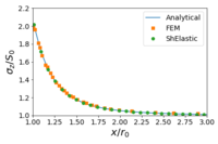
(a) Case 1
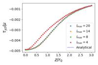
(b) Case 2
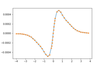
(c) Case 3


